Widrow-Hoff Learning

Preliminaries

1. ‘Performance Surfaces and Optimum Points’
2. Linear algebra
3. stochastic approximation
4. Probability Theory

ADALINE, LMS, and Widrow-Hoff learning¹

Performance learning had been discussed. But we have not used it in any neural network. In this post, we talk about an important application of performance learning. And this new neural network was invented by Frank Widrow and his graduate student Marcian Hoff in 1960. It was almost the same time as Perceptron was developed which had been discussed in ‘Perceptron Learning Rule’.

It is called Widrow-Hoff Learning. This is an approximate steepest descent algorithm. And the performance index used in the learning rule is mean square error.

Perceptron was discussed because it is still used in the current tasks. And it’s a kind of basic block of a current neural network as well. However, Widrow-Hoff learning was supposed to be discussed because it is:

1. widely used in many signal processing
2. and precursor to the backpropagation algorithm which is a very important tool of current deep learning research.

ADALINE (Adaptive LInear NEuron) and a learning rule called LMS(Least Mean Square) algorithm were introduced in the paper ‘Adaptive switching circuits’. The only distinction between perceptron and ADALINE is only the transfer function which in perceptron is a hard-limiting but in ADALINE is linear. And they have the same inherent limitation: they can only deal with the linear separable problem.

And the learning rule LMS algorithm is more powerful than the perceptron learning rule. The perceptron learning algorithm always gives a decision boundary through a training point(a sample of the training set)or near a training point as we have talked about in ‘Perceptron Learning Rule’. So this classification is not strong enough, and LMS can fix this problem. LMS had great success in signal processing but it did not work well in adapting the algorithm to the multilayer network. Backpropagation is a descendant of the LMS algorithm.

ADALINE Network

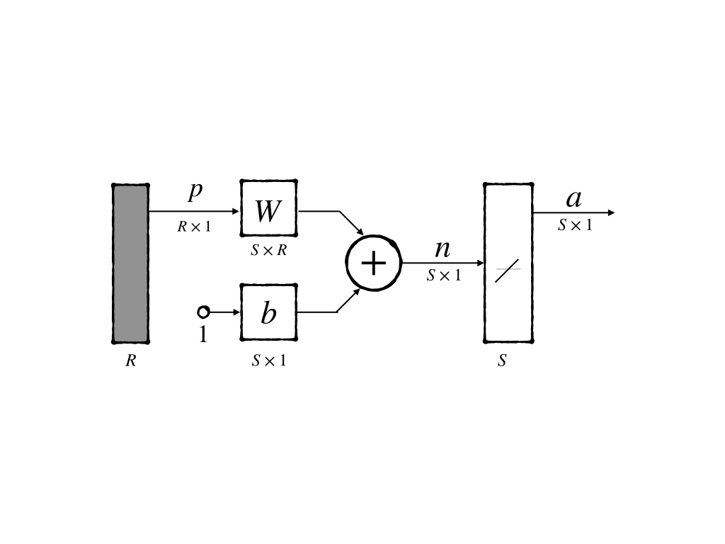
It’s an abbreviated notation of ADALINE network is;

It can be notated mathematically as: \[ \begin{aligned} \mathbf{a}&=\text{pureline}(W\mathbf{p} + \mathbf{b})\\ &= W\mathbf{p}+\mathbf{b} \end{aligned}\tag{1} \]

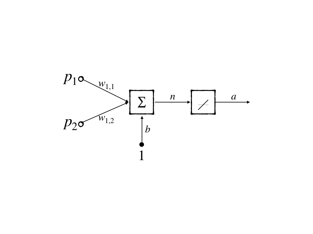
This is already a simple model, but we would like to use a more simplified model: a neuron with 2-inputs. Its abbreviated notation is:

whose mathematical notation is:

\[ \begin{aligned} \mathbf{a}&= W\mathbf{p}+\mathbf{b}\\ &=w_{1,1}p_1+w_{1,2}p_2+b \end{aligned}\tag{2} \]

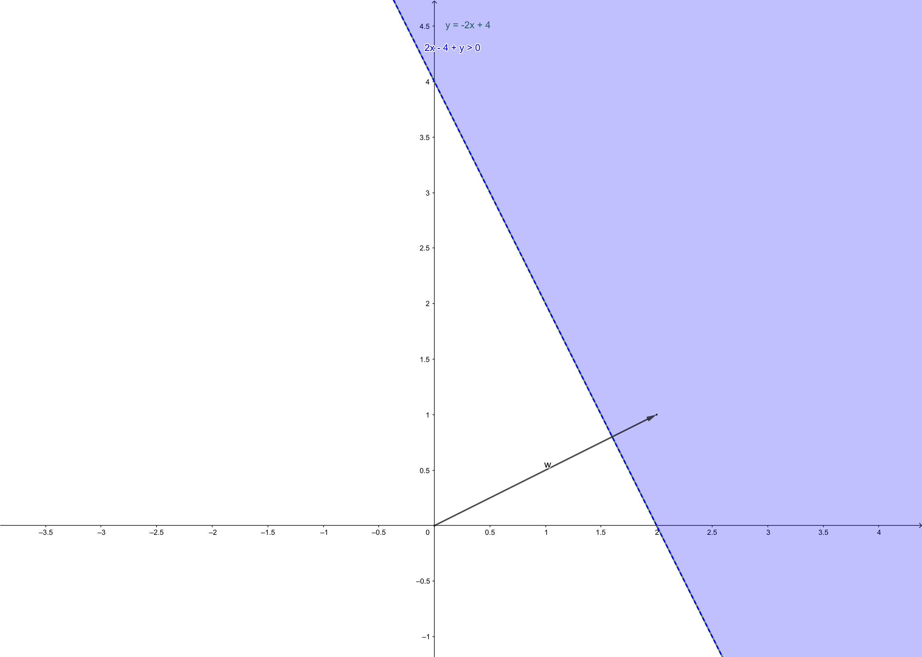
and decision boundary of this 2-input neuron is:

\(\mathbf{w}\) is the vector consisting of the weights in neuron. And it always point to the region where \(w_{1,1}p_1+w_{1,2}p_2+b>0\)

This is the simplest ADALINE neural network architecture, and then we would like to investigate ‘how to modify its parameter’ - its learning rule.

Mean Square Error

LMS is a kind of supervised learning algorithm and it needs a training set:

\[ \{\mathbf{p}_1,t_1\},\{\mathbf{p}_2,t_2\},\cdots,\{\mathbf{p}_Q,t_Q\}\tag{3} \]

And we used the information of the interaction between the output of the neural network of a certain input \(\mathbf{p}_i\) and its corresponding target \(t_i\)

The information used in LMS is the mean square error(MSE), which is the difference between output and target. This is the performance index of the ADALINE neural network.

To make the calculating process more beautiful, we lump the parameters up including bias into:

\[ \mathbf{x}=\begin{bmatrix} _1\mathbf{w}\\ b \end{bmatrix}\tag{4} \]

and input lump up respectively:

\[ \mathbf{z}=\begin{bmatrix} \mathbf{p}\\ 1 \end{bmatrix}\tag{5} \]

\(\mathbf{x}\) is used to refer to as a parameter to make it successive with the posts about performance optimization(‘Performance Surfaces and Optimum Points’) and equation(1) became:

\[ a=W\mathbf{p}+\mathbf{b}=\mathbf{x}^T\mathbf{z}\tag{6} \]

Expression for the ADALINE network mean square error:

\[ F(x)=\mathbb {E}[e^2]=\mathbb {E}[(t-a)^2]=\mathbb {E} [(t-\mathbf{x}^T\mathbf{z})^2]\tag{7} \]

where the symbol \(\mathbb{E}\) is the expectation(or average of a certain training set). Average is also called mean and the mean of the square of error so it is called MSE.

\[ \mathbb{E}[(t-\mathbf{x}^T\mathbf{z})^2]=\mathbb{E}[t^2]-2\mathbf{x}^T\mathbb{E}[t\mathbf{z}]+\mathbf{x}^T\mathbb{E}[\mathbf{z}^T\mathbf{z}]\mathbf{x}\tag{8} \]

where \(\mathbf{x}\) and \(t\) is not a random variable so its expectation is itself. And equation(8) can be simplified as

\[ F(\mathbf{x})=C-2\mathbf{x}^T\mathbf{h}+\mathbf{x}^TR\mathbf{x}\tag{9} \]

where:

• \(\mathbf{h}=t\mathbf{z}\) in statistical view, this is a cross-correlation between input and output.
• \(R=\mathbb{E}[\mathbf{z}\mathbf{z}^T]\) is input correlation matrix whose diagonal iters are mean square value of input.
• \(C=\mathbb{E}[t^2]\) is a constant.

equation(9) is a ‘quadratic function’. and we can rewrite it in the form:

\[ F(\mathbf{x})=C+ \mathbf{d}^T\mathbf{x}+\frac{1}{2}\mathbf{x}^TA\mathbf{x}\tag{10} \]

where:

• \(C=C\)
• \(\mathbf{d}^T=2\mathbf{h}^T\)
• \(A=2R=2\mathbb{E}[\mathbf{z}\mathbf{z}^T]\) is positive definite or positive semidefinite matrix. So this means the square error function could have:
  1. a strong minimum if \(R\) is positive definite and could also have a weak minimum or
  2. no minimum if \(R\) is positive semidefinite.

Then the stationary point could be at the point: \[ \nabla F(\mathbf{x})=-2\mathbf{h}+2R\mathbf{x}=0\tag{11} \]

And finally, we get the minimum point of MSE:

\[ \mathbf{x}^{\star}=R^{-1}\mathbf{h}\tag{12} \]

because \(R\) is comprised of inputs, so inputs decides the matrix \(R\) and \(R\) decides the minimum of MSE \(\mathbf{x}^{\star}\). This means when we have no information on the Hessian matrix of the performance index, our inputs are used to comprise the approximation of the Hessian matrix.

LMS Algorithm

LMS is the short for least mean square. And it is the algorithm for searching the minimum of the performance index.

When \(\mathbf{h}\) and \(R\) are known, stationary points can be found directly. If \(R^{-1}\) is impossible to calculate we can use ‘steepest descent algorithm’. However, in common both \(\mathbf{h}\) and \(R\) are unknown or are not convenient to be calculated. We would use the approximate steepest descent in which we use an estimated gradient.

And we also instead expectation of square error with a squared error:

\[ \hat{F}(\mathbf{x})=(t(k)-a(k))^2=e^2(k)\tag{13} \]

and the approximation of gradient is:

\[ \hat{\nabla}F=\nabla e^2(k)\tag{14} \]

This is the key point of the algorithm and it is also known as ‘stochastic gradient’. And when this approximation is used in a gradient descent algorithm it is referred to as

• on-line learning
• incremental learning

which means parameters are updated as each input reaches.

In the \(\nabla e^2(k)\), the first \(R\) components are the parts decided by the weights. So we have:

\[ [\nabla e^2(k)]_j=\frac{\partial e^2(k)}{\partial w_{1,j}}=2 e(k)\frac{\partial e(k)}{\partial w_{1,j}}\tag{15} \]

for \(j=1,2,\cdots, R\) and similarly

\[ [\nabla e^2(k)]_{j+1}=\frac{\partial e^2(k)}{\partial b}=2 e(k)\frac{\partial e(k)}{b}\tag{16} \]

now we consider \(\frac{\partial e(k)}{\partial w_{1,j}}\) whose error is the difference between the output of ADALINE neuron with \(R\) weights and target:

\[ \begin{aligned} \frac{\partial e(k)}{\partial w_{1,j}}&=\frac{\partial[t(k)-a(k)]}{\partial w_{1,j}}\\ &=\frac{\partial}{\partial w_{1,j}}[t(k)-(_1W^T\mathbf{p}(k)+b)]\\ &=\frac{\partial}{\partial w_{1,j}}[t(k)-(\sum_{i=1}^Rw_{1,i}p_i(k)+b)] &=-p_j(k) \end{aligned}\tag{17} \]

and similarly: \[ \frac{\partial e(k)}{b} = -1\tag{18} \]

and \(\mathbf{z}\) is conprised of \(p_j{k}\) and \(1\) as we mentioned above, so the equation(14) can be rewritten as:

\[ \hat{\nabla}F=\nabla e^2(k)=-2e(k)\mathbf{z}(k)\tag{19} \]

equation(19) gives us a beautiful form of the approximation of the gradient of squared error who is also an approximation of mean squared error.

Then we take the approximation of \(\nabla F\) into the steepest descent algorithm:

\[ \mathbf{x}_{k+1}=\mathbf{x}_{k}-\alpha \hat{\nabla} F(\mathbf{x})\bigg |_{\mathbf{x}=\mathbf{x}_k^{\star}}\tag{20} \]

and take \(\hat{\nabla} F = -2e(k)\mathbf{z}(k)\) into equation(20):

\[ \mathbf{x}_{k+1}=\mathbf{x}_{k}+2\alpha e(k)\mathbf{z}(k)\tag{21} \]

This is an LMS algorithm which is also known as the delta rule and Widrow-Hoff Learning algorithm. For multiple neuron neural networks, we have a matrix form:

\[ W(k+1)=W(k)+2\alpha \mathbf{e}(k) \mathbf{p}^T(k)\tag{22} \]

Analysis of Convergence

We have analyzed the convergence of the steepest descent algorithm, when

\[ \alpha<\frac{2}{\lambda_{\text{max}}}\tag{23} \]

and to LMS, \(\mathbf{x}(k)\) is a function of \(\mathbf{z}(k-1),\cdots \mathbf{z}(0)\) and we assume \(\mathbf{z}(k-1),\cdots \mathbf{z}(0)\) are statistical independent and \(\mathbf{x}(k)\) is independent to \(\mathbf{z}(k)\) statistically.

Because what we have used is an approximation of the steepest descent algorithm which guarantees to converge to \(\mathbf{x}^{\star}=R^{-1}\mathbf{h}\) for equation(9) and what we should do is to proof LMS converge to \(\mathbf{x}^{\star}=R^{-1}\mathbf{h}\) as well.

The update procedure of LMS is:

\[ \mathbf{x}_{k+1}=\mathbf{x}_{k}+2\alpha e(k)\mathbf{z}(k)\tag{24} \]

The expectation of both sides of equation(24):

\[ \mathbb{E}[\mathbf{x}_{k+1}]=\mathbb{E}[\mathbf{x}_{k}]+2\alpha \mathbb{E}[e(k)\mathbf{z}(k)]\tag{25} \]

substitude \(t(k)-\mathbf{x}_k^T\mathbf{z}(k)\) for the error \(e(k)\) and get:

\[ \mathbb{E}[\mathbf{x}_{k+1}]=\mathbb{E}[\mathbf{x}_{k}]+2\alpha \mathbb{E}[(t(k)-\mathbf{x}_k^T\mathbf{z}(k))\mathbf{z}(k)] \tag{26} \]

substitude \(\mathbf{z}^T(k)\mathbf{x}_k\) for \(\mathbf{x}^T_k\mathbf{z}(k)\) and rearrange terms to:

\[ \mathbb{E}[\mathbf{x}_{k+1}]=\mathbb{E}[\mathbf{x}_{k}]+2\alpha \{\mathbb{E}[t(k)\mathbf{z}(k)]-\mathbb{E}[\mathbf{z}(k)\mathbf{z}^T(k)\mathbf{x}_k]\} \tag{27} \]

because \(\mathbf{x}_k\) is independent of \(\mathbf{z}(k)\):

\[ \mathbb{E}[\mathbf{x}_{k+1}]=\mathbb{E}[\mathbf{x}_{k}]+2\alpha \{\mathbf{h}-R\mathbb{E}[\mathbf{x}_k]\} \tag{28} \]

and this can also be written as:

\[ \mathbb{E}[\mathbf{x}_{k+1}]=[I-2\alpha R]\mathbb{E}[\mathbf{x}_{k}]+2\alpha \mathbf{h} \tag{29} \]

this is also a dynamic system and to make it stable, eigenvalues of \(I-2\alpha R\) should be greater than \(-1\) and less than \(1\). And this form of the matrix has the same eigenvectors of \(R\) and its eigenvalues are \(1-2\alpha \lambda_i\) so:

\[ \begin{aligned} 1>1-2\alpha\lambda_i>&-1\\ 0<\alpha<&\frac{1}{\lambda_i} \end{aligned}\tag{30} \]

equation(30) is equivalent to:

\[ \alpha<\frac{1}{\lambda_\text{max}}\tag{31} \]

Because of \(A=2R\) so equation (31) gives the same condition as ‘steepest descent algorithm’

Under this condition, when the system becomes stable, we would have:

\[ \mathbb{E}[\mathbf{x}_{\text{ss}}]=[I-2\alpha R]\mathbb{E}[\mathbf{x}_{\text{ss}}] +2 \alpha \mathbf{h} \tag{32} \]

or

\[ \mathbb{E}[\mathbf{x}_{\text{ss}}]=R^{-1}\mathbf{h}=\mathbf{x}^{\star} \tag{33} \]

Equation(33) shows that the LMS solution which is generated by each incoming input from time to time would finally give a convergence solution.

References

Demuth, H.B., Beale, M.H., De Jess, O. and Hagan, M.T., 2014. Neural network design. Martin Hagan.↩︎