The Backpropagation Algorithm

Preliminaries

1. An Introduction to Backpropagation and Multilayer Perceptrons
2. Culculus 1,2
3. Linear algebra
4. Jacobian matrix

Architecture and Notations¹

We have seen a three-layer network is flexible in approximating functions(An Introduction to Backpropagation and Multilayer Perceptrons). If we had a more-than-three-layer network, it could be used to approximate any functions as accurately as we want. However, another trouble that came to us is the learning rules. This problem almost killed neural networks in the 1970s. Until the backpropagation(BP for short) algorithm was found that it is an efficient algorithm in training multiple layers networks.

A 3-layer network is also used in this post for it is the simplest multiple-layer network whose abbreviated notation is:

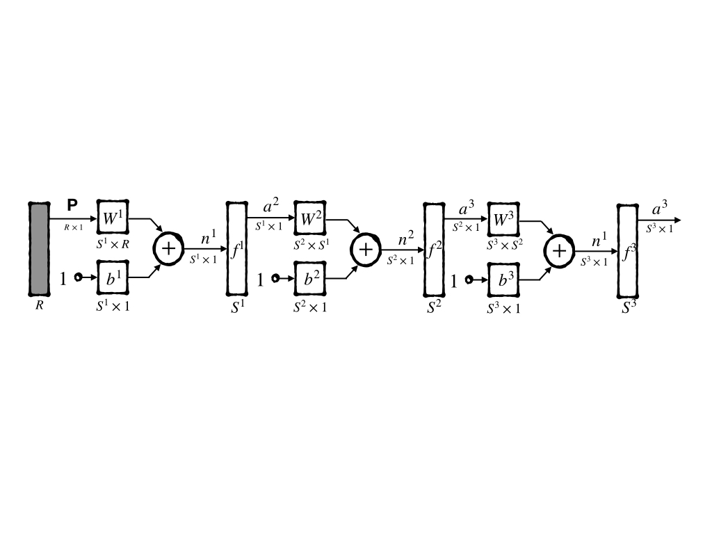
and a more short way to represent its architecture is:

\[ R - S^1 - S^2 - S^3 \tag{1} \]

For the three-layer network has only three layers that are not too large to denote mathematically, then it can be written as:

\[ \mathbf{a}=f^3(W^3\cdot f^2(W^2\cdot f^1(W^1\cdot \mathbf{p}+\mathbf{b}^1)+\mathbf{b}^2)+\mathbf{b}^3)\tag{2} \]

However, this mathematical equation is too complex to construct when we have a 10-layer network or a 100-layer network. Then we can use some short equations that describe the whole operation of the \(M\)-layer network:

\[ a^{m+1}=f^{m+1}(W^{m+1}\mathbf{a}^{m}+\mathbf{b}^{m+1})\tag{3} \]

for \(m = 1, 2, 3, \cdots M-1\). \(M\) is the number of layers in the neural networks. And: - \(\mathbf{a}^0=\mathbf{p}\) is its input - \(\mathbf{a}=\mathbf{a}^M\) is its output

Performance Index

We have had a network now. Then we need to definite a performance index for this 3-layer network.

MSE is used here as the performance index the same as what the LMS algorithm did in post ‘Widrow-Hoff Learning’. And the training set is:

\[ \{\mathbf{p}_1,\mathbf{t}_1\},\{\mathbf{p}_2,\mathbf{t}_2\},\cdots \{\mathbf{p}_Q,\mathbf{t}_Q\}\tag{4} \]

where \(\mathbf{p}_i\) is the input and \(\mathbf{t}_i\) is the corresponding output(target).

BP is the generation of LMS algorithms, and both of them try to minimize the mean square error. And what we finally get is a trained neural network that fits the training set. But this model may not be guaranteed to fit the original task where the training set is generated. So a good training set that can represent the original task accurately is necessary.

To make it easier to understand from the steepest descent algorithm to LMS and BP, we convert the weights and bias in the neural network form \(w\) and \(b\) into a vector \(\mathbf{x}\). Then the performance index is:

\[ F(\mathbf{x})=\mathbb E[e^2]=\mathbb E[(t-a)^2]\tag{5} \]

When the network has multiple outputs this generalizes to:

\[ F(\mathbf{x})=\mathbb E[\mathbf{e}^T\mathbf{e}]=\mathbb E[(\mathbf{t}-\mathbf{a})^T(\mathbf{t}-\mathbf{a})]\tag{6} \]

During an iteration, in the LMS algorithm, MSE(mean square error) is approximated by SE(square error):

\[ \hat{F}(\mathbf{x})=(\mathbf{t}-\mathbf{a})^T(\mathbf{t}-\mathbf{a})=\mathbf{e}^T\mathbf{e}\tag{7} \]

where the expectations are replaced by the calculation of current input, output, and target.

Reviewing the ‘steepest descent algorithm’, the gradient descent algorithm of approximate MSE is also called stochastic gradient descent:

\[ \begin{aligned} w^m_{i,j}(k+1)&=w^m_{i,j}(k)-\alpha \frac{\partial \hat{F}}{\partial w^m_{i,j}}\\ b^m_{i}(k+1)&=b^m_{i}(k)-\alpha \frac{\partial \hat{F}}{\partial b^m_{i}} \end{aligned}\tag{8} \]

where \(\alpha\) is the learning rate.

However, the steep descent algorithm seems can not work on a multiple-layer network for we can not calculate the partial derivative in the hidden layer and input layer directly.

We were inspired by another mathematical tool - the chain rule.

The Chain Rule

Calculus

when \(f\) is explicit function of \(\mathbf{n}\) and \(\mathbf{n}\) is a explicit function of \(\mathbf{w}\), we can calculate the partial derivative \(\frac{\partial f}{\partial w}\) by:

\[ \frac{\partial f}{\partial w}=\frac{\partial f}{\partial n}\frac{\partial n}{\partial w}\tag{9} \]

The whole process looks like a chain. And let’s look at a simple example: when we have \(f(n)=e^n\) and \(n=2w\), we have \(f(n(w))=e^{2w}\). We can easily calculate the direvative \(\frac{\partial f}{\partial w}=\frac{\partial e^2w}{\partial w}=2e^{2w}\). And when chain rule is used, we have:

\[ \frac{\partial f(n(w))}{\partial w}=\frac{\partial e^n}{\partial n}\frac{\partial n}{\partial w}=\frac{\partial e^n}{\partial n}\frac{\partial 2w}{\partial w}=e^n\cdot 2=2e^{2w}\tag{10} \]

that is the same as what we get directly.

When the chain rule is used in the second part on the right of equation (8), we get the way to calculate the derivative of the weight of hidden layers:

\[ \begin{aligned} \frac{\partial \hat{F}}{\partial w^m_{i,j}}&=\frac{\partial \hat{F}}{\partial n^m_i}\cdot \frac{\partial n^m_i}{\partial w^m_{i,j}}\\ \frac{\partial \hat{F}}{\partial b^m_{i}}&=\frac{\partial \hat{F}}{\partial n^m_i}\cdot \frac{\partial n^m_i}{\partial b^m_{i}} \end{aligned}\tag{11} \]

from the abbreviated notation, we know that \(n^m_i=\sum^{S^{m-1}}_{j=1}w^m_{i,j}a^{m-1}_{j}+b^m_i\). Then equation (11) can be writen as:

\[ \begin{aligned} \frac{\partial \hat{F}}{\partial w^m_{i,j}}&=\frac{\partial \hat{F}}{\partial n^m_i}\cdot \frac{\partial \sum^{S^{m-1}}_{j=1}w^m_{i,j}a^{m-1}_{j}+b^m_i}{\partial w^m_{i,j}}=\frac{\partial \hat{F}}{\partial n^m_i}\cdot a^{m-1}_j\\ \frac{\partial \hat{F}}{\partial b^m_{i}}&=\frac{\partial \hat{F}}{\partial n^m_i}\cdot \frac{\partial \sum^{S^{m-1}}_{j=1}w^m_{i,j}a^{m-1}_{j}+b^m_i}{\partial b^m_{i}}=\frac{\partial \hat{F}}{\partial n^m_i}\cdot 1 \end{aligned}\tag{12} \]

Equation (12) could also be simplified by defining a new concept: sensitivity.

Sensitivity

We define sensitivity as \(s^m_i\equiv \frac{\partial \hat{F}}{\partial n^m_{i}}\) that means the sensitivity of \(\hat{F}\) to changes in the \(i^{\text{th}}\) element of the net input at layer \(m\). Then equation (12) can be simplified as:

\[ \begin{aligned} \frac{\partial \hat{F}}{\partial w^m_{i,j}}&=s^m_{i}\cdot a^{m-1}_j\\ \frac{\partial \hat{F}}{\partial b^m_{i}}&=s^m_{i}\cdot 1 \end{aligned}\tag{13} \]

Then the steepest descent algorithm is: \[ \begin{aligned} w^m_{i,j}(k+1)&=w^m_{i,j}(k)-\alpha s^m_{i}\cdot a^{m-1}_j\\ b^m_{i}(k+1)&=b^m_{i}(k)-\alpha s^m_{i}\cdot 1 \end{aligned}\tag{14} \]

This can also be written in a matrix form:

\[ \begin{aligned} W^m(k+1)&=W^m(k)-\alpha \mathbf{s}^m(\mathbf{a}^{m-1})^T\\ \mathbf{b}^m(k+1)&=\mathbf{b}^m(k)-\alpha \mathbf{s}^m\cdot 1 \end{aligned}\tag{15} \]

where: \[ \mathbf{s}^m=\frac{\partial \hat{F}}{\alpha \mathbf{n}^m}=\begin{bmatrix} \frac{\partial \hat{F}}{\partial n^m_1}\\ \frac{\partial \hat{F}}{\partial n^m_2}\\ \vdots\\ \frac{\partial \hat{F}}{\partial n^m_{S^m}}\\ \end{bmatrix}\tag{16} \]

And be careful of the \(\mathbf{s}\) which means the sensitivity and \(S^m\) which means the number of layers \(m\)

Backpropagating the Sensitivities

Equation (15) is our BP algorithm. But we can not calculate sensitivities yet. We can easily calculate the sensitivities of the last layer which is the same as LMS. And we have an inspiration that is we can use the relation between the latter layer and the current layer. So let’s observe the Jacobian matrix which represents the relation between the latter layer linear combination output \(\mathbf{n}^{m+1}\) and the current layer linear combination output \(\mathbf{n}^m\):

\[ \frac{\partial \mathbf{n}^{m+1}}{\partial \mathbf{n}^{m}}= \begin{bmatrix} \frac{ \partial n^{m+1}_1}{\partial n^{m}_1} & \frac{\partial n^{m+1}_1}{\partial n^{m}_2} & \cdots & \frac{\partial n^{m+1}_1}{\partial n^{m}_{S^m}}\\ \frac{\partial n^{m+1}_2}{\partial n^{m}_1} & \frac{\partial n^{m+1}_2}{\partial n^{m}_2} & \cdots & \frac{\partial n^{m+1}_2}{\partial n^{m}_{S^m}}\\ \vdots&\vdots&&\vdots\\ \frac{\partial n^{m+1}_{S^{m+1}}}{\partial n^{m}_1} & \frac{\partial n^{m+1}_{S^{m+1}}}{\partial n^{m}_2} & \cdots & \frac{\partial n^{m+1}_{S^{m+1}}}{\partial n^{m}_{S^m}}\\ \end{bmatrix}\tag{17} \]

And the \((i,j)^{\text{th}}\) element of the matrix is:

\[ \begin{aligned} \frac{\partial n^{m+1}_i}{\partial n^{m}_j}&=\frac{\partial (\sum^{S^m}_{l=1}w^{m+1}_{i,l}a^m_l+b^{m+1}_i)}{\partial n^m_j}\\ &= w^{m+1}_{i,j}\frac{\partial a^m_j}{\partial n^m_j}\\ &= w^{m+1}_{i,j}\frac{\partial f^m(n^m_j)}{\partial n^m_j}\\ &= w^{m+1}_{i,j}\dot{f}^m(n^m_j) \end{aligned}\tag{18} \]

where \(\sum^{S^m}_{l=1}w^{m+1}_{i,l}a^m_l+b^{m+1}_i\) is the linear combination output of layer \(m+1\) and \(a^m\) is the output of layer \(m\). And we can define \(\dot{f}^m(n^m_j)=\frac{\partial f^m(n^m_j)}{\partial n^m_j}\)

Therefore the Jacobian matrix can be written as:

\[ \begin{aligned} &\frac{\partial \mathbf{n}^{m+1}}{\partial \mathbf{n}^{m}}\\ =&W^{m+1}\dot{F}^m(\mathbf{n}^m)\\ =&\begin{bmatrix} w^{m+1}_{1,1}\dot{f}^m(n^m_1) & w^{m+1}_{1,2}\dot{f}^m(n^m_2) & \cdots & w^{m+1}_{1,{S^m}}\dot{f}^m(n^m_{S^m})\\ w^{m+1}_{2,1}\dot{f}^m(n^m_1) & w^{m+1}_{2,2}\dot{f}^m(n^m_2) & \cdots & w^{m+1}_{2,{S^m}}\dot{f}^m(n^m_{S^m})\\ \vdots&\vdots&&\vdots\\ w^{m+1}_{S^{m+1},1}\dot{f}^m(n^m_1) & w^{m+1}_{S^{m+1},2}\dot{f}^m(n^m_2) & \cdots & w^{m+1}_{S^{m+1},{S^m}}\dot{f}^m(n^m_{S^m}) \end{bmatrix} \end{aligned} \tag{19} \]

where we have:

\[ \dot{F}^m(\mathbf{n}^m)= \begin{bmatrix} \dot{f}(n^m_1)&0&\cdots&0\\ 0&\dot{f}(n^m_2)&\cdots&0\\ \vdots&\vdots&\ddots&\vdots\\ 0&0&\cdots&\dot{f}(n^m_{S^m}) \end{bmatrix}\tag{20} \]

Then recurrence relation for the sensitivity by using the chain rule in matrix form is:

\[ \begin{aligned} \mathbf{s}^m&=\frac{\partial \hat{F}}{\partial n^m}\\ &=(\frac{\partial \mathbf{n}^{m+1}}{\partial \mathbf{n}^{m}})^T\cdot \frac{\partial \hat{F}}{\partial n^{m+1}}\\ &=\dot{F}^m(\mathbf{n}^m)W^{m+1}\mathbf{s}^{m+1}\\ \end{aligned}\tag{21} \]

This is why it is called backpropagation because the sensitivities of layer \(m\) are calculated by layer \(m+1\) :

\[ S^{M}\to S^{M-1}\to S^{M-2}\to \cdots \to S^{1}\tag{22} \]

Same to the LMS algorithm, BP is also an approximating algorithm of the steepest descent technique. And the start of BP \(\mathbf{s}^M_i\) is:

\[ \begin{aligned} \mathbf{s}^M_i&=\frac{\partial \hat{F}}{\partial n^m_i}\\ &=\frac{\partial (\mathbf{t}-\mathbf{a})^T(\mathbf{t}-\mathbf{a})}{\partial n^m_i}\\ &=\frac{\partial \sum_{j=1}^{S^M}(t_j-a_j)^2}{\partial n^M_i}\\ &=-2(t_i-a_i)\frac{\partial a_i}{\partial n^M_{i}} \end{aligned}\tag{23} \]

and this is easy to understand because it is just a variation of the LMS algorithm. Since

\[ \frac{\partial a_i}{\partial n^M_i}=\frac{\partial f^M(n^M_i)}{\partial n^M_i}=\dot{f}^M(n^M_j)\tag{24} \]

we can write:

\[ s^M_i=-2(t_i-a_i)\dot{f}^M(n^M_i)\tag{25} \]

and its matrix form is:

\[ \mathbf{s}^M_i=-\dot{F}^M(\mathbf{n}^M)(\mathbf{t}-\mathbf{a})\tag{26} \]

Summary of BP

1. Propagate the input forward through the network
   • \(\mathbf{a}^0=\mathbf{p}\)
   • \(\mathbf{a}^{m+1}=f^{m+1}(W^{m+1}\mathbf{a}^m+\mathbf{b}^{m+1})\) for \(m=0,1,2,\cdots, M-1\)
   • \(\mathbf{a}=\mathbf{a}^M\)
2. Propagate the sensitivities backward through the network:
   • \(\mathbf{s}^M=-2\dot{F}^M(\mathbf{n}^M)(\mathbf{t}-\mathbf{a})\)
   • \(\mathbf{s}^m= \dot{F}^m(\mathbf{n}^m)(W^{m+1})^T\mathbf{s}^{m+1})\) for \(m=M-1,\cdots,2,1\)
3. Finally, the weights and bias are updated using the approximate steepest descent rule:
   • \(W^{m}(k+1)=W^{m}(k)-\alpha \mathbf{s}^m(\mathbf{a}^{m-1})^T\)
   • \(\mathbf{b}^{m}(k+1)=\mathbf{b}^{m}(k)-\alpha \mathbf{s}^m\)

References

Demuth, Howard B., Mark H. Beale, Orlando De Jess, and Martin T. Hagan. Neural network design. Martin Hagan, 2014.↩︎