Steepest Descent Method

Preliminaries

1. ‘An Introduction to Performance Optimization’
2. Linear algebra
3. Calculus 1,2

Direction Based Algorithm and a Variation¹

This post describes a direction searching algorithm(\(\mathbf{x}_{k}\)). And its variation gives a way to estimate step length (\(\alpha_k\)).

Steepest Descent

To find the minimum points of a performance index by an iterative algorithm, we want to decrease the value of the performance index step by step which looks like going down from the top of the hill. And the crucial of this algorithm is that every iteration makes the performance index decrease:

\[ F(\mathbf{x}_{k+1})<F(\mathbf{x}_{k})\tag{1} \]

Our mission is to find the direction \(\mathbf{p}_k\) with a relatively short step length \(\alpha_k\) which leads us downhill.

The first-order Taylor series of an iterative step is:

\[ F(\mathbf{x}_{k+1})=F(\mathbf{x}_{k}+\Delta \mathbf{x}_k)\approx F(\mathbf{x}_{k})+\mathbf{g}^T\Delta\mathbf{x}_k\tag{2} \]

where \(\mathbf{g}_k\) is the gradient at position \(\mathbf{x}\) of the performance index \(F(\mathbf{x})\) which means:

\[ \mathbf{g}_k = \nabla F(\mathbf{x})\bigg |_{\mathbf{x}=\mathbf{x}_k}\tag{3} \]

From equation(1) and equation(2) for the purpose \(F(\mathbf{x}_{k+1})<F(\mathbf{x}_{k})\), we need:

\[ \mathbf{g}^T\Delta\mathbf{x}_k<0\tag{4} \]

( \(\Delta\mathbf{x}_k\) , the change of \(\mathbf{x}_k\), can also be represented by step length \(\alpha_k\) and direction \(\mathbf{p}\), then the equation(4) has a equivalent form:

\[ \alpha_k\mathbf{g}^T\Delta\mathbf{p}_k<0\tag{5} \]

In the previous posts, we have seen how to find the greatest value of \(\mathbf{g}^T\Delta\mathbf{p}_k\). And now we can find the smallest value of \(\mathbf{g}^T\Delta\mathbf{p}_k\) in the same way. Then we got the smallest value is:

\[ -\mathbf{g}^T\mathbf{g}\tag{6} \]

which means that the deepest direction we would search is:

\[ \Delta\mathbf{p}_k=-\mathbf{g}\tag{7} \]

According to the iterative optimization algorithm framework in‘An Introduction to Performance Optimization’, the second step is :

\[ \mathbf{x}_{k+1}=\mathbf{x}_{k}-\alpha_k\mathbf{g}_k\tag{8} \]

The step length is also called the learning rate. And the choice of \(\alpha_k\) can be:

1. Minimizing \(F(\mathbf{x})\) with \(\alpha_k\) by minimizing along the line: \(\mathbf{x}_k-\alpha_k\mathbf{g}_k\)
2. Fixed \(\alpha_k\), such as \(\alpha_k=0.002\)
3. Predetermined, like \(\alpha_k=\frac{1}{k}\)

An Example

\[ F(\mathbf{x})=x_1^2+25x_2^2\tag{9} \]

1. start at point \(x=\begin{bmatrix}0.5\\0.5\end{bmatrix}\)
2. gradient of \(F(\mathbf{x})\) is \(\nabla F(\mathbf{x})=\begin{bmatrix}\frac{\partial F}{\partial x_1}\\\frac{\partial F}{\partial x_2}\end{bmatrix}=\begin{bmatrix}2x_1\\50x_2\end{bmatrix}\)
3. \(\mathbf{g}_0=\nabla F(\mathbf{x})\bigg|_{\mathbf{x}=\mathbf{x}_0}=\begin{bmatrix}1\\25\end{bmatrix}\)
4. set \(\alpha = 0.01\)
5. update: \(\mathbf{x}_1=\mathbf{x}_0-0.01\mathbf{g}_0=\begin{bmatrix}0.5\\0.5\end{bmatrix}-0.01\begin{bmatrix}1\\25\end{bmatrix}=\begin{bmatrix}0.49\\0.25\end{bmatrix}\)
6. update: \(\mathbf{x}_2=\mathbf{x}_1-0.01\mathbf{g}_1=\begin{bmatrix}0.49\\0.25\end{bmatrix}-0.01\begin{bmatrix}0.98\\12.5\end{bmatrix}=\begin{bmatrix}0.4802\\0.125\end{bmatrix}\)
7. go on updating until the smallest point is achieved.

The whole trajectory looks like this:

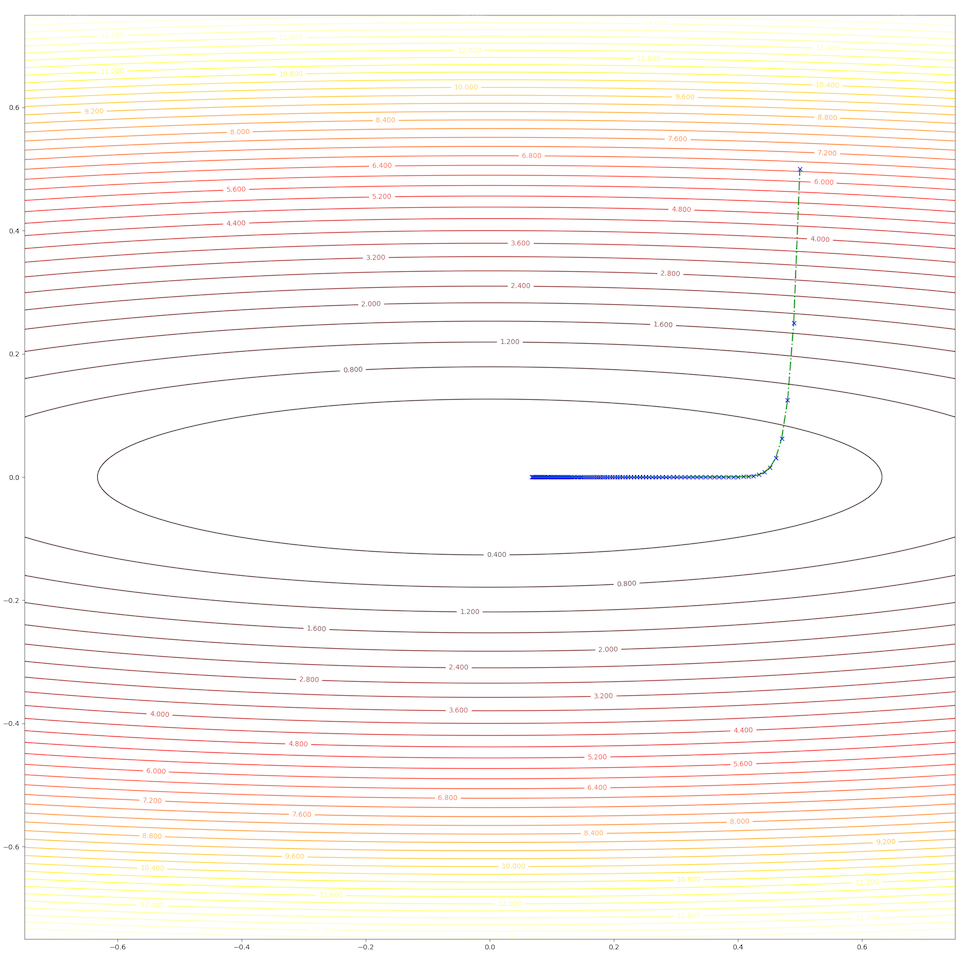
and the learning rate, step length is a constant in this algorithm, however, we can test 2 different values and watch their behavior. When we set \(\alpha=0.01\), we have:

and when we set \(\alpha=0.02\), we have:

These results illustrated:

1. In first several steps, the descent speed is faster than in later steps
2. A greater learning rate seems to have a higher speed
3. This algorithm can converge to the minimum point.

The second point gives us a new idea, of what will the algorithms do when we have a relatively bigger learning rate. To be on the safe side we select a not so big learning rate \(\alpha=0.05\), we have:

this algorithm diverges, which means it would never stop at the minimum and get farther and farther as steps go on. So we have to take care of the value of the learning rate, a small learning rate can slow down the algorithm but a big one can break up the algorithm.

Stable Learning Rates

To have a fast speed and converge to the minimum, we need to study the learning rate \(\alpha\). To simplify the problem, we start with supposing the performance index is a quadratic function:

\[ F(\mathbf{x})=\frac{1}{2}\mathbf{x}^TA\mathbf{x}+\mathbf{d}^T\mathbf{x}+c\tag{10} \]

and we have already known its gradient is:

\[ \nabla F(\mathbf{x})=A \mathbf{x}+\mathbf{d}\tag{11} \]

we take equation(11) into update step equation(8), we have:

\[ \mathbf{x}_{k+1}=\mathbf{x}_k-\alpha\mathbf{g}_k=\mathbf{x}_k-\alpha(A \mathbf{x}_k+\mathbf{d})\tag{12} \]

or an equivalent form:

\[ \mathbf{x}_{k+1}=(I-\alpha A)\mathbf{x}_k - \alpha\mathbf{d}\tag{13} \]

In the linear algebra course or other courses, this equation is called a ‘linear dynamic system’. To make the system stable, the eigenvalues of \(I-\alpha A\) are less than one in magnitude. And \(I-\alpha A\) has the same eigenvectors with \(A\). Let \([\lambda_1,\lambda_2,\cdots,\lambda_n]\) be the eigenvalues of \(A\) and let \([\mathbf{z}_1,\mathbf{z}_2,\cdots,\mathbf{z}_n]\) be the eigenvectors of \(A\)

\[ [I-\alpha A]\mathbf{z}_i=\mathbf{z}_i-\alpha A\mathbf{z}_i=\mathbf{z}_i-\alpha \lambda_i\mathbf{z}_i=(1-\alpha\lambda_i)\mathbf{z}_i\tag{14} \]

\(I-\alpha A\) has the same eigenvectors with \(A\) and has the eigenvalues: \([1-\alpha\lambda_1,1-\alpha\lambda_2,\cdots,1-\alpha\lambda_n]\)

Concerning the equation(13) and eigenvalues of \(I-\alpha A\) to stabilize the system which here is the steepest descent algorithm, we need:

\[ \begin{aligned} &|1-\alpha \lambda_i|&<1\\ -1&<1-\alpha \lambda_i&<1\\ -2&<-\alpha \lambda_i&<0\\ \end{aligned}\tag{15} \]

for \(\alpha>0\)

\[ \begin{aligned} \frac{2}{\alpha}&> \lambda_i&>0\\ \end{aligned}\tag{16} \]

from equation(16), we finally have \[ \frac{2}{\lambda_i}>\alpha\tag{17} \]

which implies:

\[ \frac{2}{\lambda_{\text{max}}}>\alpha\tag{18} \]

This gives us the maximum stable learning rate is inversely proportional to the maximum curvature(direction along with eigenvector according to the maximum eigenvalue \(\lambda_\text{max}\)) of the quadratic function.

Let’s go back to the example, the Hessian matrix of the equation(9) is: \[ A=\begin{bmatrix} 2&0\\0&50 \end{bmatrix}\tag{19} \]

its eigenvectors and eigenvalues are: \[ \{\lambda_1=2,\mathbf{z}_1=\begin{bmatrix}1\\0\end{bmatrix}\},\{\lambda_2=50,\mathbf{z}_2=\begin{bmatrix}0\\1\end{bmatrix}\}\tag{20} \]

taking \(\lambda_\text{max}=\lambda_2=50\) into equation(18), we get: \[ \alpha_\text{max}<\frac{2}{50}=0.04\tag{21} \]

so, let’s check the behavior of the algorithm when \(\alpha=0.039\) and \(\alpha=0.041\):

1. set \(\alpha=0.039\) we have:
2. set \(\alpha=0.041\) we have:

Up to now, both concepts and implements have been built to prove the correctness of the algorithm. And we also have the following tips:

1. The algorithm tends to converge most quickly in the direction of the eigenvector corresponding to the largest eigenvalue
2. The algorithm tends to converge most slowly in the direction of the eigenvector corresponding to the smallest eigenvalue
3. Do not overshoot the minimum point for the too-long step(learning rate \(\alpha\))

Minimizing along a Line

The section above gives us the upper bound of \(\alpha\), but we have three kinds of strategies for selecting a \(\alpha\).

The first one is “Minimizing \(F(\mathbf{x})\) with \(\alpha_k\) by minimizing along the line: \(\mathbf{x}_k-\alpha_k\mathbf{g}_k\)”. What shall we do with this kind of \(\alpha\)?

To arbitrary functions, the stationary point along a direction can be calculated by:

\[ \begin{aligned} &\frac{dF}{d\alpha_k}(\mathbf{x}_k+\alpha_k\mathbf{p}_k)\\ &=\nabla F(\mathbf{x})^T\bigg|_{\mathbf{x}=\mathbf{x}_k}\mathbf{p}_k+\alpha_k\mathbf{p}_k^T\nabla F^2(\mathbf{x})^T\bigg|_{\mathbf{x}=\mathbf{x}_k}\mathbf{p}_k\\ &=0 \end{aligned}\tag{22} \]

and then

\[ \alpha=-\frac{\nabla F(\mathbf{x})^T\bigg|_{\mathbf{x}=\mathbf{x}_k}\mathbf{p}_k}{\mathbf{p}_k^T\nabla F^2(\mathbf{x})\bigg|_{\mathbf{x}=\mathbf{x}_k}\mathbf{p}_k}=-\frac{\mathbf{g}^T_k\mathbf{p}_k}{\mathbf{p}_k^TA_k\mathbf{p}_k}\tag{23} \]

where: \(A_k\) is the Hessian matrix of an old guess \(\mathbf{x}_k\):

\[ A_k=\nabla^2F(\mathbf{x})\bigg|_{\mathbf{x}=\mathbf{x}_k}\tag{24} \]

Here we look at an example:

\[ F(x)=\frac{1}{2}\mathbf{x}^T\begin{bmatrix} 2&1\\1&2 \end{bmatrix}\mathbf{x}\tag{25} \]

with the initial guess \[ \mathbf{x}_0=\begin{bmatrix}0.8\\-0.25\end{bmatrix}\tag{26} \]

the gradient of the function is

\[ \nabla F(\mathbf{x})=\begin{bmatrix}2x_1+x_2\\x_1+2x_2\end{bmatrix}\tag{27} \]

the initial direction of the algorithm is

\[ \mathbf{p}_0=-\mathbf{g}_0=-\nabla F(\mathbf{x})\bigg|_{\mathbf{x}=\mathbf{x}_k}=\begin{bmatrix}-1.35\\-0.3\end{bmatrix}\tag{28} \]

and take equation(28) and \(A=\begin{bmatrix}2&1\\1&2\end{bmatrix}\) into equation(23): \[ \alpha_0=\frac{\begin{bmatrix}1.35&0.3\end{bmatrix}\begin{bmatrix}2&1\\1&2\end{bmatrix}}{\begin{bmatrix}1.35&0.3\end{bmatrix}\begin{bmatrix}2&1\\1&2\end{bmatrix}\begin{bmatrix}1.35\\0.3\end{bmatrix}}=0.413\tag{29} \]

and take all these data into equation(8):

\[ \mathbf{x}_1=\mathbf{x}_0-\alpha_0\mathbf{g}_0=\begin{bmatrix}0.8\\-0.25\end{bmatrix}-0.413\begin{bmatrix}1.35\\0.3\end{bmatrix}=\begin{bmatrix}0.24\\-0.37\end{bmatrix}\tag{30} \]

What is going on is repeating the steps: equation(26) to equation(30) until some terminative conditions are achieved. It works like this:

All the new directions in the steps are orthogonal to their last direction:

\[ \mathbf{p}_{k+1}^T\mathbf{p}_k=\mathbf{g}_{k+1}^T\mathbf{p}_k=0\tag{31} \]

what we need now is to proof is \(\mathbf{g}_{k+1}^T\mathbf{p}_k=0\), with the chain rule of equation(22):

\[ \begin{aligned} \frac{d}{d\alpha_k}F(\mathbf{x}_{k+1})&=\frac{d}{d\alpha_k}F(\mathbf{x}_k+\alpha_k\mathbf{p}_k)\\ &=\nabla F(\mathbf{x})^T\bigg|_{\mathbf{x}=\mathbf{x}_{k+1}}\frac{d}{d\alpha_k}(\mathbf{x}_k+\alpha_k\mathbf{p}_k)\\ &=\nabla F(\mathbf{x})^T\bigg|_{\mathbf{x}=\mathbf{x}_{k+1}}\mathbf{p}_k\\ &=0 \end{aligned}\tag{32} \]

equation(32) gives us: a new direction is always orthogonal to the last step direction at the minimum point of the function along the last step direction. This is also an inspiration for another algorithm called conjugate direction.

References

Demuth, H.B., Beale, M.H., De Jess, O. and Hagan, M.T., 2014. Neural network design. Martin Hagan.↩︎