Quadratic Functions

Preliminaries

1. Linear algebra
2. Calculus 1,2
3. Taylor series

Quadratic Functions¹

Quadratic function, a type of performance index, is universal. One of its key properties is that it can be represented in a second-order Taylor series precisely.

\[ F(\mathbf{x})=\frac{1}{2}\mathbf{x}^TA\mathbf{x}+\mathbf{d}\mathbf{x}+c\tag{1} \]

where \(A\) is a symmetric matrix(if it is not symmetric, it can be easily converted into symmetric). And recall the property of gradient:

\[ \nabla (\mathbf{h}^T\mathbf{x})=\nabla (\mathbf{x}^T\mathbf{h})=\mathbf{h}\tag{2} \]

and

\[ \nabla (\mathbf{x}^TQ\mathbf{x})=Q\mathbf{x}+Q^T\mathbf{x}=2Q\mathbf{x}\tag{3} \]

then the first order of quadratic functions are:

\[ \nabla F(\mathbf{x})=A\mathbf{x}+\mathbf{d}\tag{4} \]

and second-order of quadratic functions are: \[ \nabla^2 F(\mathbf{x})=A\tag{5} \]

The shape of quadratic functions can be described by eigenvalues and eigenvectors of its Hessian matrix. Hessian matrix is a symmetric matrix and its eigenvectors are mutually orthogonal, let:

\[ \mathbf{z}_1,\mathbf{z}_2,\cdots ,\mathbf{z}_n\tag{6} \]

denote the whole set of the eigenvectors of the Hessian matrix \(A\) and we build a matrix:

\[ B=\begin{bmatrix} \mathbf{z}_1&\mathbf{z}_2&\cdots &\mathbf{z}_n \end{bmatrix}\tag{7} \]

and because of \(BB^T=I\), we have \(B^{-1}=B^T\). When the Hessian matrix is positive definite, it would have \(n\) eigenvectors(Hessian has a full rank \(n\)) and we can change the Hessian matrix into a new matrix whose basis are the set of eigenvectors:

\[ A'=B^TAB=\begin{bmatrix} \lambda_1&&&\\ &\lambda_2&&\\ &&\ddots&\\ &&&\lambda_n \end{bmatrix}=\Lambda\tag{8} \]

after changing the basis, the new Hessian matrix is a diagonal matrix whose elements on the diagonal are the eigenvalues. This process can be inversed because of \(BB^T=I\):

\[ A=BA'B^T=B\Lambda B^T\tag{9} \]

We can calculate the derivative in any directions:

\[ \frac{\mathbf{p}^T\nabla^2 F(\mathbf{x})\mathbf{p}}{||\mathbf{p}||^2}=\frac{\mathbf{p}^TA\mathbf{p}}{||\mathbf{p}||^2}\tag{10} \]

For columns of \(B\) can span the whole space, So we can find a vector \(\mathbf{c}\) satisfy:

\[ \mathbf{p}=B\mathbf{c}\tag{11} \]

then take equation(8), equation(11) into equation(10) we get:

\[ \frac{\mathbf{c}^TB^TAB\mathbf{c}}{\mathbf{c}^TB^TB\mathbf{c}}=\frac{\mathbf{c}^T\Lambda\mathbf{c}}{\mathbf{c}^TI\mathbf{c}}=\frac{\sum^n_{i=1}\lambda_i c_i^2}{\sum_{i=1}^n c^2_i}\tag{12} \]

From equation(12), we could conclude:

\[ \lambda_{\text{min}}\leq \frac{\mathbf{p}^TA\mathbf{p}}{||\mathbf{p}||^2}\leq \lambda_{\text{max}}\tag{13} \]

1. maximum \(2^{\text{nd}}\) derivative occure along with \(\mathbf{z}_{\text{max}}\)(according to \(\lambda_{\text{max}}\))
2. eigenvalues is the \(2^{\text{nd}}\) derivative along its eigenvector.
3. eigenvectors could define a new coordinate system
4. eigenvectors are principal axes of the function contour.
5. going along with the \(\mathbf{z}_{\text{max}}\) direction could have the largest change in function value \(|\Delta F(x)|\)
6. eigenvalues here are all positive because of positive definite.

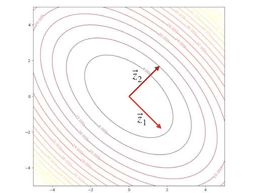
An example:

\[ F(\mathbf{x})=x_1^2+x_1x_2+x_2^2 =\frac{1}{2}\mathbf{x}^T \begin{bmatrix} 2&1\\1&2 \end{bmatrix}\mathbf{x}\tag{14} \]

we can calculate the eigenvectors and eigenvalues:

\[ \begin{aligned} &\lambda_1=1&&\mathbf{z}_1=\begin{bmatrix} 1\\-1 \end{bmatrix}\\ &\lambda_2=3&&\mathbf{z}_2=\begin{bmatrix} 1\\1 \end{bmatrix} \end{aligned}\tag{15} \]

The contour plot and 3-D plots are:

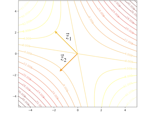
Another example:

\[ F(\mathbf{x})=-\frac{1}{4}x_1^2-\frac{3}{2}x_1x_2-\frac{1}{4}x_2^2 =\frac{1}{2}\mathbf{x}^T \begin{bmatrix} -0.5&-1.5\\-1.5&-0.5 \end{bmatrix}\mathbf{x}\tag{16} \]

we can calculate the eigenvectors and eigenvalues:

\[ \begin{aligned} &\lambda_1=1&&\mathbf{z}_1=\begin{bmatrix} -1\\1 \end{bmatrix}\\ &\lambda_2=-2&&\mathbf{z}_2=\begin{bmatrix} -1\\-1 \end{bmatrix} \end{aligned}\tag{17} \]

The contour plot and 3-D plots is:

Conclusion

1. \(\lambda_i>0\) or \(i=1,2,\cdots\), \(F(x)\) have a single strong minimum
2. \(\lambda_i<0\) or \(i=1,2,\cdots\), \(F(x)\) have a single strong maximum
3. \(\lambda_i\) have both negative and positive together. \(F(x)\) has a saddle point
4. \(\lambda_i\geq 0\) and have a \(\lambda_j=0\), \(F(x)\) has a weak minimum or has no stationary point.
5. \(\lambda_i\leq 0\) and have a \(\lambda_j=0\), \(F(x)\) has a weak maximum or has no stationary point.

References

Demuth, H.B., Beale, M.H., De Jess, O. and Hagan, M.T., 2014. Neural network design. Martin Hagan.↩︎