Newton's Method

Preliminaries

1. ‘steepest descent algorithm’
2. Linear Algebra
3. Calculus 1,2

Newton’s Method¹

Taylor series gives us the conditions for minimum points based on both first-order items and the second-order item. And first-order item approximation of a performance index function produced a powerful algorithm for locating the minimum points which we call ‘steepest descent algorithm’.

Now we want to have an insight into the second-order approximation of a function to find out whether there is an algorithm that can also work as a guide to the minimum points. The approximation of \(F(\mathbf{x}_{k+1})\) is:

\[ \begin{aligned} F(\mathbf{x}_{k+1})&=F(\mathbf{x}_k+\Delta \mathbf{x}_k)\\ &\approx F(\mathbf{x}_k)+\mathbf{g}^T_k\Delta \mathbf{x}_k+\frac{1}{2}\Delta \mathbf{x}^T_kA_k\Delta \mathbf{x}_k \end{aligned} \tag{1} \]

Now we replace the performance index with its Taylor approximation in equation 1. The gradient of equation 1:

\[ \nabla F(\mathbf{x}_{k+1})=A_k\mathbf{x}_k+\mathbf{g}_k\tag{2} \]

To get the stationary points, we set equation(2) equal to \(0\):

\[ \begin{aligned} A_k\Delta \mathbf{x}_k+\mathbf{g}_k&=0\\ \Delta \mathbf{x}_k&=-A_k^{-1}\mathbf{g}_k \end{aligned} \tag{3} \]

then as the iterative algorithm framework said, we update \(\mathbf{x}_k\) which is also known as Newton’s Method:

\[ \mathbf{x}_{k+1}=\mathbf{x}_k+\Delta \mathbf{x}_k=\mathbf{x}_k-A_k^{-1}\mathbf{g}_k\tag{4} \]

Now is the time to look at an example:

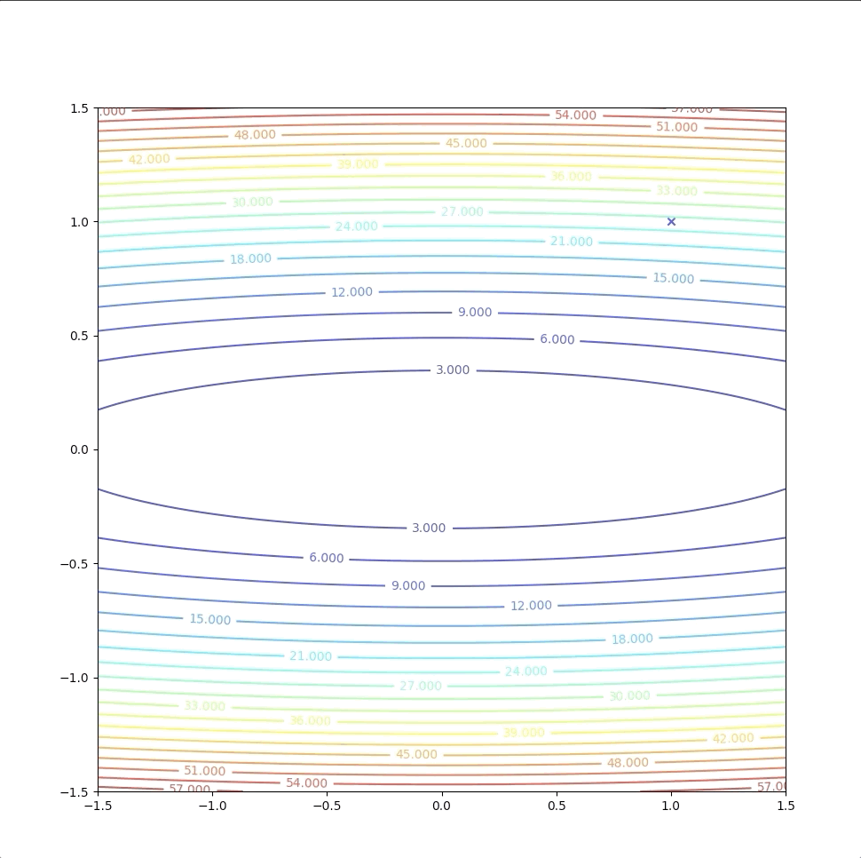
\[ F(\mathbf{x})=x^2_1+25x_2^2\tag{5} \]

the gradient of equation(5) is:

\[ \nabla F(\mathbf{x})= \begin{bmatrix} \frac{\partial}{\partial x_1}F(\mathbf{x})\\ \frac{\partial}{\partial x_2}F(\mathbf{x}) \end{bmatrix}= \begin{bmatrix} 2x_1\\ 50x_2 \end{bmatrix}\tag{6} \]

the Hessian matrix is:

\[ \nabla F(\mathbf{x})= \begin{bmatrix} \frac{\partial^2}{\partial^2 x_1}F(\mathbf{x})& \frac{\partial^2}{\partial x_1 \partial x_2}F(\mathbf{x})\\ \frac{\partial^2}{\partial x_2\partial x_1}F(\mathbf{x})&\frac{\partial^2}{\partial^2 x_2}F(\mathbf{x}) \end{bmatrix}= \begin{bmatrix} 2&0\\ 0&50 \end{bmatrix}\tag{7} \]

then we update \(\mathbf{x}\) as equation(4) and with the intial point \(\mathbf{x}_0=\begin{bmatrix}1\\1\end{bmatrix}\)

\[ \begin{aligned} \mathbf{x}_1&=\mathbf{x}_0-A_k^{-1}\mathbf{g}_k\\ &=\begin{bmatrix}1\\1\end{bmatrix}-\begin{bmatrix}0.5&0\\0&0.02\end{bmatrix}\begin{bmatrix}2\\50\end{bmatrix}\\ &=\begin{bmatrix}0\\0\end{bmatrix} \end{aligned} \tag{8} \]

Then we test \(\mathbf{x}_{1}=\begin{bmatrix}0\\0\end{bmatrix}\) with terminational condition. And then we stop this algorithm.

This one-step algorithm is not a coincidence. This method will always find the minimum of a quadratic function in 1 step. This is because the second-order approximation of the quadratic function is just itself in another form. They have the same minimum and stationary points. However, when \(F(x)\) is not quadratic the method may:

1. not generally converge in 1 step and
2. be not sure whether the algorithm could converge or not which is dependent on both the performance index and the initial guess.

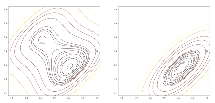
Let’s consider a function that is not quadratic:

\[ F(\mathbf{x})=(x_2-x_1)^4 + 8x_1x_2-x_1+x_2+3\tag{9} \]

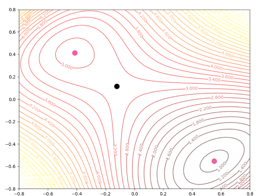
There are a local minimum, a global minimum, and a saddle point.

With the initial point \(\mathbf{x}_0=\begin{bmatrix}1.5\\0\end{bmatrix}\)

Then we keep updating the position \(\mathbf{x}_k\) with the equation(4) and we have:

The right side of the figure is the process of second-order Taylor approximation.

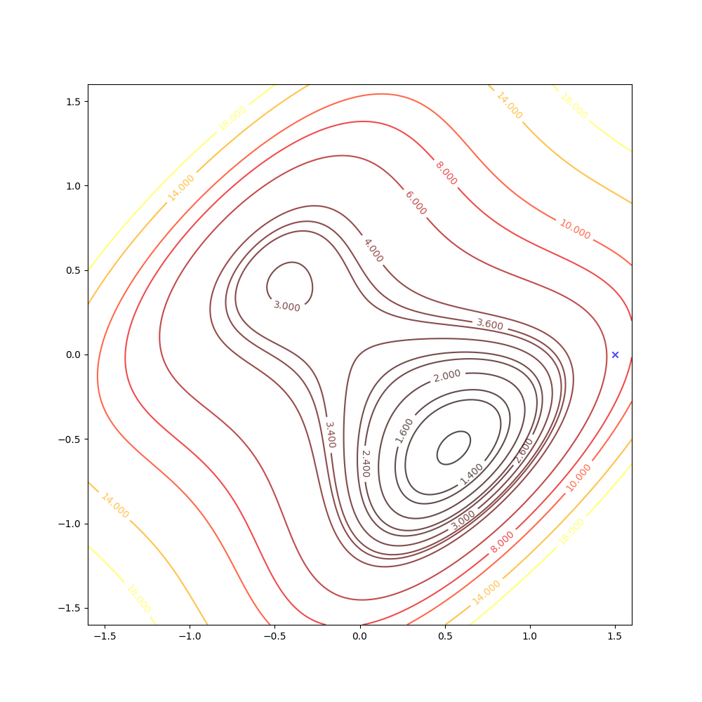
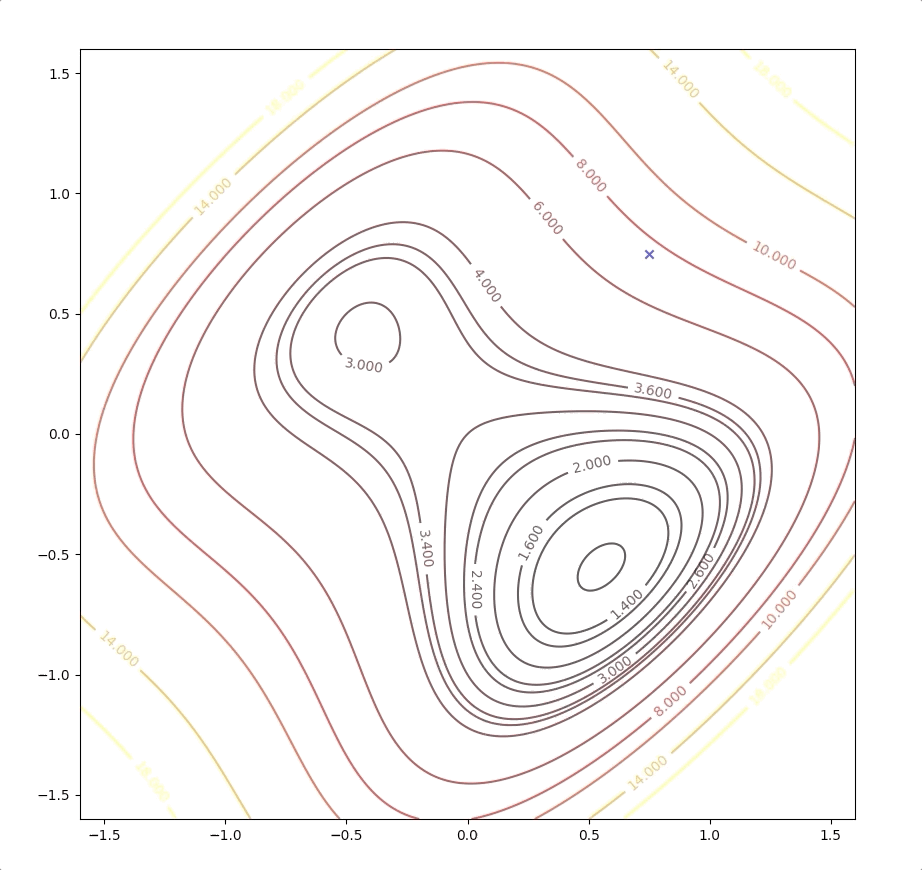
if we initial the process at the point \(\mathbf{x}_0=\begin{bmatrix}0.75\\0.75\end{bmatrix}\). It will be looked like:

The right side of the figure is the process of second-order Taylor approximation.

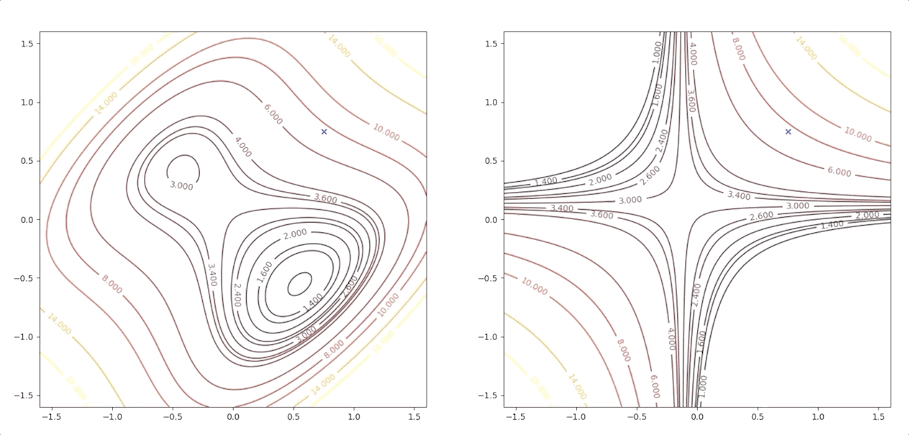
and it converges to the saddle point.

Newton’s method converges quickly in many applications. The analytic function can be accurately approximated by quadratic in a small neighborhood of a strong minimum. And Newton’s method can not distinguish between local minimum, global minimum, and saddle points.

When we use a quadratic function approximation, we consider the quadratic function only and forget the other parts of the original function where it is not able to be approximated by the quadratic function. So what we can see through a quadratic approximate is only a small region where there is only one minimum. We can not distinguish which kind of stationary point it is. And Newton’s method can produce very unpredictable results, too.

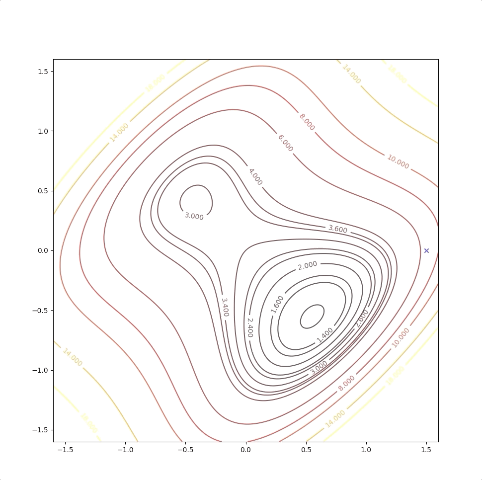
If the initial point is \(\mathbf{x}_0=\begin{bmatrix}1.15\\0.75\end{bmatrix}\) of the example above, it is far from the minimum but it finally converges to the minimum point :

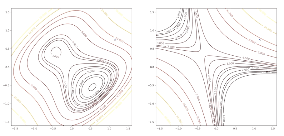
while the initial point \(\mathbf{x}_0=\begin{bmatrix}0.75\\0.75\end{bmatrix}\) which is more close to the minimum converge to the saddle points:

the right side of the figure is the process of second-order Taylor approximation.

Conclusion

Newton’s method is:

1. faster than the steepest descent
2. quite complex
3. possible oscillate or diverge (steepest descent is guaranteed to converge when the learning rate is suitable)
4. and there is a variation of Newton’s method suited to neural networks.
5. the computation and storage of the Hessian matrix and its inverse could easily exhaust our computational resource
6. Newton’s method degenerates to the steepest descent method when \(A_k=A_k^{-1}=I\)

References

Demuth, H.B., Beale, M.H., De Jess, O. and Hagan, M.T., 2014. Neural network design. Martin Hagan.↩︎