Neuron Model and Network Architecture

Preliminaries

1. linear classifier
2. An Introduction to Neural Networks

Theory and Notation¹

We are not able to build any artificial cells up to now. It seems impossible to build a neuron network through biological materials manually, either. To investigate the ability of neurons we have built mathematical models of the neuron. These models have been assigned a number of neuron-like properties. However, there must be a balance between the number of properties contained by the mathematical models and the current computational abilities of the machines.

From now on, we begin our study of the neuron network, and it looks like a good idea, to begin with, the simplest but basic model – artificial neuron. Because tons of network architectures are built on these simple neurons.

Single Neuron Model

Let’s begin with the simplest neuron, which has only one input, one synapse which is represented by weight, a bias, a threshold operation which is expressed by a transfer function, and an output.

We know that the cell body of neurons plays summation and threshold operation. This is very like a linear classifier

Then our simplest model is constructed as follows:

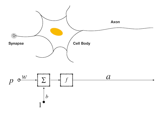
1. Synapse is represented by a scalar which is called a weight, it will be multiplied by the input as a received signal, and then the signal is transferred to the cell body
2. Cell body here is represented by two functional properties property:
   • the first one is summation which is used to collect all signals in a short time interval, while in this naive example only one input is concerned so it looks redundant but in the following models, it is an important operation of a neuron;
   • the second function is a threshold operation that acts as a gatekeeper, only the signal stronger than some value could excite this neuron. Only excited neurons could pass signals to the other neurons connected to them.
3. and a scalar
   • The scalar property represents an original faint signal of the neuron. From a biological point, it makes sense because every nerve cell has its resting membrane potential(RMP).
4. Axon is expressed by an output that is produced by the threshold function. It can be any form in a biological neuron, like amplitude or frequency, but here it can just be a number that is decided by the selected threshold function.

The threshold function is called an active function or transfer functions officially. And it will be listed in the next section.

Let’s review the single input neuron model and its components:

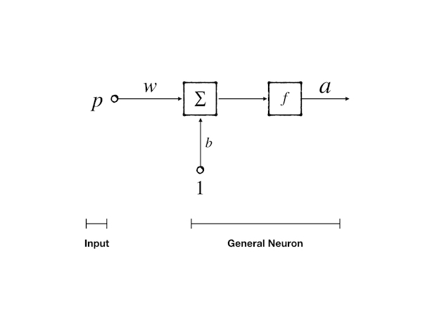
• \(P\): input signal, a scalar or vector, coming from a previous nerve cell or external signal
• \(w\): weight, a scalar or vector, coming from the synapse, act as the strength of a synapse
• \(b\): bias, a scalar, a property of this neuron
• \(f\): transfer function, act as a gatekeeper, perform a threshold operation
• \(a\): the output of the neuron, a scalar, can be a signal to the next neuron or as a final output to the external system.

The final mathematical expression is:

\[ a=f(w\cdot P + b)\tag{1} \]

For instance, we have input \(P=2.0\), synapse weight \(w=3.0\), nerve cell bias \(b=-1.5\) and then we get the output:

\[ a= f(2.0\times 3.0 + (-1.5))=f(4.5)\tag{2} \]

however, bias can be omitted, or be rewritten as a special input and weight combination:

\[ a=f(w_1\cdot P + w_0\cdot 1)\text{ where } w_1=w \text{ and }w_0=b\tag{3} \]

\(w\) and \(b\) came from equation(1). In the model, \(w\) and \(b\) are adjustable. And the ideal procedure is: 1. computing summation of all weighted inputs 2. select a transfer function 3. put the result of step 1 into the selected function from step 2 and get a final output of the neuron 4. using the learning rule to adjust \(w\) and \(b\) to adapt the task which is our purpose.

Transfer Functions

Every part of the neuron no matter the biological or mathematical one directly affects the function of the neuron. And this also makes the design of neurons more interesting, because we can build different kinds of neurons to simulate different kinds of operations. And this also provides sufficient basic blocks for us to develop a more complicated network.

Let’s recall the single input model above, the components are \(w\), \(b\), \(\sum\), and \(f\), however, \(w\) and \(b\) are objectives of learning, and \(\sum\) is relatively stable which is hard to be replaced by any other operations. So, we move our attention to the threshold operation-\(f\). Threshold operation is like a switch that when some conditions are achieved produces a special output. But when the conditions are not reached, it gives another output. A simple mathematical equation to express this function is:

\[ f(x) = \begin{cases} 0, & \text{if $x>0$} \\ 1, & \text{else} \end{cases}\tag{4} \]

Transfer functions can be linear or nonlinear; the Following three functions are mostly used.

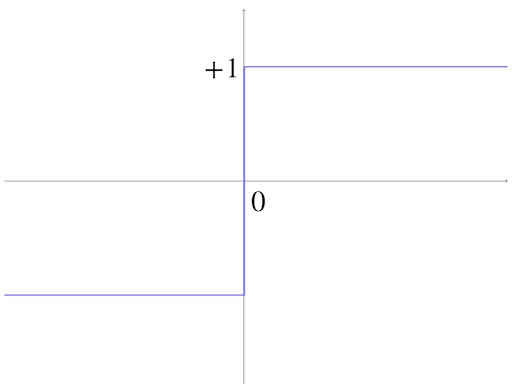
Hard Limit Transfer Function

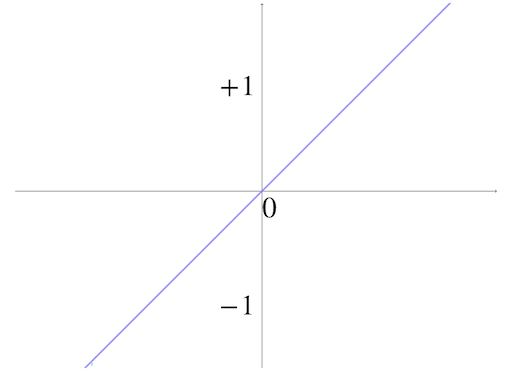
The first commonly used threshold function is the most intuitive one, a piecewise function, when \(x>0\) the output is ‘on’ or ‘off’ for others. And by convention, ‘on’ is replaced by \(1\) and ‘off’ is replaced by \(-1\). So it becomes:

\[ f(x) = \begin{cases} 1, & \text{if $x>0$} \\ -1, & \text{else} \end{cases}\tag{5} \]

and it looks like this:

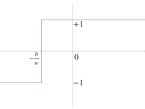
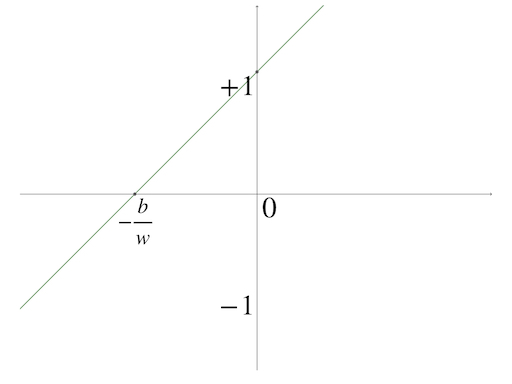
Then we take equation(1) into equation(5), we get: \[ f(w\cdot P +b) = \begin{cases} 1, & \text{if $w\cdot P +b>0$} \\ -1, & \text{else} \end{cases}\tag{6} \]

We always regard the input as an independent variable so we replace \(P\) with \(x\) without loss of generality. Then we get:

\[ g(x) = \begin{cases} 1, & \text{if $x> -\frac{b}{w}$} \\ -1, & \text{else} \end{cases}\tag{7} \]

where \(w\neq 0\). \(g(x)\) is a special case for equation(5) as the transfer function of this single-input neuron.

This is the famous threshold operation function, the Hard Limit Transfer Function

Linear Transfer Function

Another mostly used function is the linear function, which has the simplest form:

\[ f(x)=x\tag{8} \]

and it is a line going through the origin

When tale equation(1) into equation(8) we get:

\[ f(w\cdot P+b)=w\cdot P+b\tag{9} \]

and we can get the special case of the linear transfer function for the single-input neuron:

\[ g(x)=w\cdot x+b\tag{10} \]

The linear transfer function just seems as if there is no transfer function in the model but in some networks, it plays an important part.

Log-sigmoid Transfer Function

Another useful transfer function is the log-sigmoid function:

\[ f(x)=\frac{1}{1+e^{-x}}\tag{11} \]

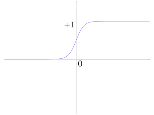
This sigmoid function has a similar appearance to the ‘Hard Limit Transfer Function’ however, the sigmoid has a more mathematical advantage than the hard limit transfer function, like it has derivative everywhere while equation(5) does not.

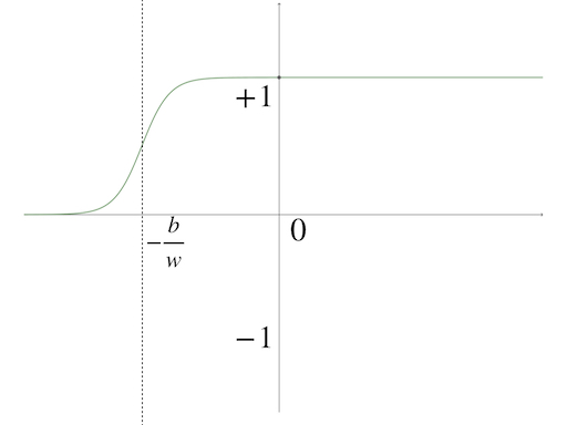
The single-input neuron model’s special case of the log-sigmoid function is:

\[ g(x)=\frac{1}{1+e^{-w\cdot x+b}}\tag{12} \]

and it looks like this:

These three transfer functions are the most common ones and also the easiest ones. More transfer functions can be found:‘Transfer Function’

Multiple-inputs Neuron

After the insight of the single-input neuron, we can easily build a more complex and powerful neuron model- a multiple-inputs neuron, whose structure is more like the biological nerve cell than the single-input neuron:

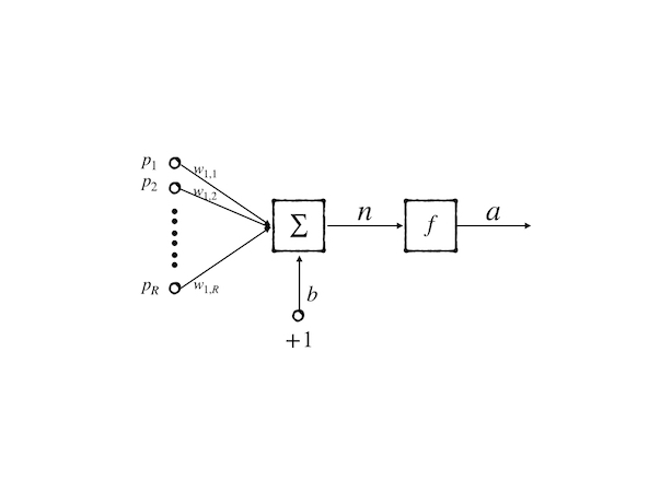
then, the mathematical expression is:

\[ a=w_{1,1}\cdot p_1+w_{1,2}\cdot p_2+\dots+ w_{1,R}\cdot p_R+b\tag{13} \]

There are two numbers of subscript of \(w\) which seem unnecessary in the equation because the first number does not vary anymore. But as a long concern, it is better to remain this number for it is used to label the neuron. So \(w_{1,2}\) represents the second synapse’s weight belonging to the first neuron. When we have \(k\) neurons the \(m\)th synapse weight of \(n\)th neuron is \(w_{n,m}\).

Let’s go back to the equation(13). It can be rewritten as:

\[ n=W\mathbf{p}+b\tag{14} \]

where: - \(W\) is a matrix that has only one row containing the weights - \(\mathbf{p}\) is a vector representing inputs - \(b\) is a scalar representing bias - \(n\) is the result of the cell body operation,

then the output is:

\[ a=f(W\mathbf{p}+b)\tag{15} \]

The diagram is a very powerful tool to express a neuron or a network because it’s good at showing the topological structure of the network. And for further research, an abbreviated notation had been designed. To the multiple-inputs neuron, we have:

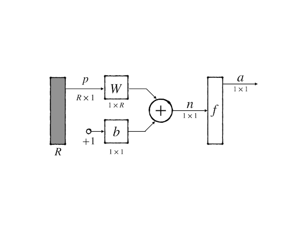
a feature of this kind of notation is that the dimensions of each variable are labeled and the input dimension \(R\) is decided by the designer.

Network Architecture

A single neuron is not sufficient, even though it has multiple inputs.

A layer of neurons

To perform a more complicated function, we need more than one neuron and construct a network that contains a layer of neurons:

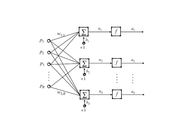
in this model, we have \(R\)-dimensions input and \(S\) neurons then we get:

\[ a_i=f(\sum_{j=1}^{R}w_{i,j}\cdot p_{j}+b_j)\tag{16} \]

this is the output of \(j\) the neuron in the whole network, and we can rewrite the whole network in a metrical form:

\[ \mathbf{a}=\mathbf{f}(W\mathbf{p}+\mathbf{b})\tag{17} \]

where

• \(W\) is a matrix \(\begin{bmatrix}w_{1,1}&\cdots&w_{1,R}\\ \vdots&&\vdots\\w_{S,1}&\cdots&w_{S_R}\end{bmatrix}\), where \(w_{i,j}\) is the \(j\)th weight of the \(i\)th neuron
• \(\mathbf{p}\) is the vector of input \(\begin{bmatrix}p_1\\ \vdots\\p_R\end{bmatrix}\)
• \(\mathbf{a}\) is the vector of output \(\begin{bmatrix}a_1\\ \vdots\\a_S\end{bmatrix}\)
• \(\mathbf{f}\) is the vector of transfer functions \(\begin{bmatrix}f_1\\ \vdots\\f_S\end{bmatrix}\) where each \(f_i\) can be different.

This network is much more powerful than the single neuron but they have a very similar abbreviated notation:

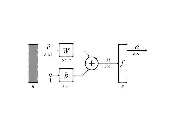
the only distinction is the dimension of each variable.

Multiple Layers of Neurons

The next stage of extending a single-layer network is multiple layers:

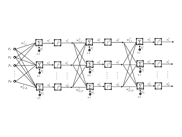
and, its final output is:

\[ \mathbf{a}=\mathbf{f}^3(W^3\mathbf{f}^2(W^2\mathbf{f}^1(W^1\mathbf{p}+\mathbf{b}^1)+\mathbf{b}^2)+\mathbf{b}^3)\tag{18} \]

the numbers on the right-top of the variable are the layer number, for example, \(w^1_{2,3}\) is the weight of \(2\) nd synapse of the \(3\) rd neuron at the 1st layer.

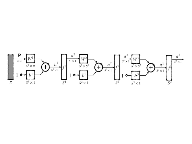
Each layer has also its name, for instance, the first layer whose input is external input is called the input layer. The layer whose output is external output is called the output layer. Other layers are called hidden layers. Its abbreviated notation is:

The new model with multiple layers is powerful but it is hard to design because the layer number is arbitrary and the neurons number in each layer is also untractable. So it becomes an experimental work. However, the input layer and output layer usually have a certain number and they are decided by the specialized task. Transfer functions are decided by the designer, and each neuron can have its transfer function different from any other neurons in the network.

Bias can be omitted but this can cause a problem that it will always output \(\mathbf{0}\) when the input is \(\mathbf{0}\). This phenomenon could not make sense in some tasks, so bias plays an important part in the \(\mathbf{0}\) input situation. But to some other input, bias seems not so important.

Recurrent Networks

It seems possible that a neuron’s output also connects to its input. It acts somehow like

\[ \mathbf{a}=\mathbf{f}(W\mathbf{f}(W\mathbf{p}+\mathbf{b})+\mathbf{b})\tag{19} \]

to illustrate the procedure, we present the delay block

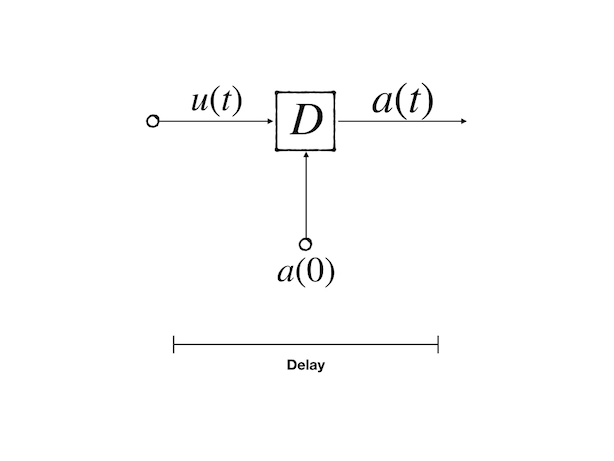
where the output is the input delayed 1-time unit:

\[ a(t)=u(t-1)\tag{20} \]

and the block is initialized by \(a(0)\)

Another useful operation for the recurrent network is integrator:

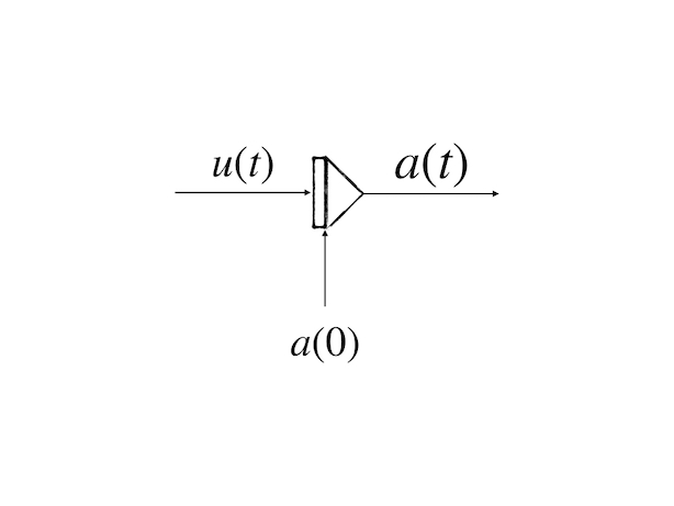
whose output is:

\[ a(t)=\int^t_0u(t)dt +a(0)\tag{21} \]

A recurrent network is a network in which there is a feedback connection. Here we just list some basic concepts and more details would be researched in the following posts. The recurrent network works more powerful than a feedforward network because it exhibits temporal behavior which is a fundamental property of the biological brain. A typical recurrent network is:

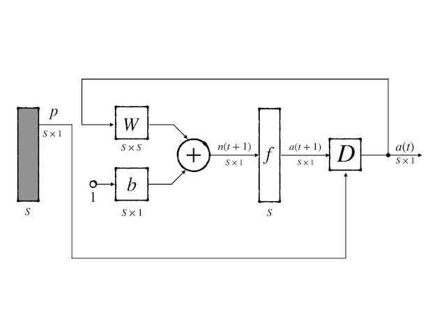
where:

\[ a(0)=\mathbf{p} \\ a(t+1)=f(W\mathbf{p}+\mathbf{b})\tag{22} \]

References

Demuth, H.B., Beale, M.H., De Jess, O. and Hagan, M.T., 2014. Neural network design. Martin Hagan.↩︎