Logistic Regression

Preliminaries

1. ‘An Introduction to Probabilistic Generative Models for Linear Classification’

Idea of logistic regression¹

Logistic sigmoid function(logistic function for short) had been introduced in post ‘An Introduction to Probabilistic Generative Models for Linear Classification’. It has an elegant form:

\[ \delta(a)=\frac{1}{1+e^{-a}}\tag{1} \]

and when \(a=0\), \(\delta(a)=\frac{1}{2}\) and this is just the half of the range of logistic function. This gives us a strong implication that we can set \(a\) equals to some functions \(y(\mathbf{x})\), and then

\[ a=y(\mathbf{x})=0\tag{2} \]

becomes a decision boundary. Here the logistic function plays the same role as the threshold function described in the post ‘From Linear Regression to Linear Classification’

Logistic Regression of Linear Classification

The easiest decision boundary is a constant corresponding to a 1-deminsional input. The dicision boundary of 1-deminsional input is a degenerated line, namely, a point. Here we consider a little complex function - a 2-deminsional input vector \(\begin{bmatrix}x_1&x_2\end{bmatrix}^T\) and the function \(y(\mathbf{x})\) is:

\[ y(\mathbf{x})=w_0+w_1x_1+w_2x_2=\mathbf{w}^T\mathbf{x}= \begin{bmatrix}w_0&w_1&w_2\end{bmatrix} \begin{bmatrix} 1\\ x_1\\ x_2 \end{bmatrix}\tag{3} \]

Then we substitute this into equation (1), we got our linear logistic regression function:

\[ y(\mathbf{x})=\delta(\mathbf{w}^T\mathbf{x})=\frac{1}{1+e^{-\mathbf{w}^T\mathbf{x}}}\tag{4} \]

The output of the equation (4) is a real number, its range is \((0,1)\). So it can be used to represent a probability of the input belonging to \(\mathcal{C}_1\) whose label is \(1\) or \(\mathcal{C}_0\) whose label is \(0\) in the training set.

Estimating the Parameters in Logistic Regression

Although logistic regression is called regression, it acts as a classifier. Our mission, now, is to estimate the parameters in equation(4).

Recalling that the output of equation(4) is \(\Pr(\mathcal{C}_1|\mathbf{x},M)\) where \(M\) is the model we selected. And the model sometimes can be represented by its parameters. And the mission should you chose to accept it, is to build probability \(\Pr(\mathbf{w}|\mathbf{x},t)\) where \(\mathbf{x}\) is the input vector and \(t\in\{0,1\}\) is the corresponding label and condition \(\mathbf{x}\) is always been omitted. \(t\) is one of \(\mathcal{C}_1\) or \(\mathcal{C}_2\), so the Bayesian relation of \(\Pr(\mathbf{w}|t)\) is:

\[ \Pr(\mathbf{w}|t)=\frac{\Pr(t|\mathbf{w})\Pr(\mathbf{w})}{\Pr(t)}=\frac{\Pr(\mathcal{C}_i|\mathbf{w})\Pr(\mathbf{w})}{\Pr(t)}=\frac{\Pr(\mathcal{C}_i|\mathbf{x},M)\Pr(\mathbf{w})}{\Pr(t)}\tag{5} \]

Then the maximum likelihood function is employed to estimate the parameters. And the likelihood is just:

\[ \Pr(\mathcal{C}_1|\mathbf{x},M)=\delta(\mathbf{w}^T\mathbf{x})=\frac{1}{1+e^{-\mathbf{w}^T\mathbf{x}}}\tag{6} \]

When we have had the training set:

\[ \{\mathbf{x}_1,t_1\},\{\mathbf{x}_2,t_2\},\cdots,\{\mathbf{x}_N,t_N\}\tag{7} \]

the likelihood becomes:

\[ \Pi_{t_i\in \mathcal{C}_1}\frac{1}{1+e^{-\mathbf{w}^T\mathbf{x_i}}}\Pi_{t_i\in \mathcal{C}_0}(1-\frac{1}{1+e^{-\mathbf{w}^T\mathbf{x_i}}})\tag{8} \]

In the second part, when \(\mathbf{x}\) belongs to \(\mathcal{C}_0\) the label is \(0\). The output of this class should approach to \(0\), so minimising \(\frac{1}{1+e^{-\mathbf{w}^T\mathbf{x_i}}}\) equals to maximising \(1-\frac{1}{1+e^{-\mathbf{w}^T\mathbf{x_i}}}\). For equation(8) is not convenient to optimise, we can use the property that \(t_n\in{0,1}\) and we have:

\[ \begin{aligned} &\Pi_{t_i\in \mathcal{C}_1}\frac{1}{1+e^{-\mathbf{w}^T\mathbf{x_i}}}\Pi_{t_i\in \mathcal{C}_0}(1-\frac{1}{1+e^{-\mathbf{w}^T\mathbf{x_i}}})\\ =&\Pi_i^N(\frac{1}{1+e^{-\mathbf{w}^T\mathbf{x_i}}})^{t_i}(1-\frac{1}{1+e^{-\mathbf{w}^T\mathbf{x_i}}})^{1-t_i} \end{aligned} \tag{9} \]

From now on, we turn to an optimization problem. Maximizing equation(9) equals to minimize its minus logarithm(we use \(y_i\) retpresent \(\frac{1}{1+e^{-\mathbf{w}^T\mathbf{x_i}}}\)):

\[ \begin{aligned} E&=-\mathrm{ln}\;\Pi^N_{i=1}y_i^{t_i}(1-y_i)^{1-t_i}\\ &=-\sum^N_{i=1}(t_i\mathrm{ln}y_i+(1-t_i)\mathrm{ln}(1-y_i)) \end{aligned} \tag{10} \]

Equation(10) is called cross-entropy, which is a very important concept in information theory and is called cross-entropy error in machine learning which is also a very useful function.

For there is no closed-form solution to the optimization problem in equation(10), ‘steepest descent algorithm’ is employed. And what we need to calculate firstly is the derivative of equation(10). For we want to get the derivative of \(\mathbf{w}\)of function \(y_i(\mathbf{x})\), the chain rule is necessary:

\[ \begin{aligned} \frac{dE}{dw}&=-\frac{d}{dw}\sum^N_{i=1}(t_i\mathrm{ln}y_i+(1-t_i)\mathrm{ln}(1-y_i))\\ &=-\sum^N_{i=1}\frac{d}{dw}t_i\mathrm{ln}y_i+\frac{d}{dw}(1-t_i)\mathrm{ln}(1-y_i)\\ &=-\sum^N_{i=1}t_i\frac{y_i'}{y_i}+(1-t_i)\frac{-y'_i}{1-y_i} \end{aligned} \tag{11} \]

and

\[ \begin{aligned} y_i'&=\frac{d}{dw}\frac{1}{1+e^{-\mathbf{w}^T\mathbf{x_i}}}\\ &=\frac{\mathbf{x}e^{-\mathbf{w}^T\mathbf{x_i}}}{(1+e^{-\mathbf{w}^T\mathbf{x_i}})^2} \end{aligned}\tag{12} \]

Substitute equation (12) into equation (11), we have:

\[ \begin{aligned} \frac{dE}{dw}&=-\sum_{i=1}^Nt_i\frac{\frac{\mathbf{x}e^{-\mathbf{w}^T\mathbf{x_i}}}{(1+e^{-\mathbf{w}^T\mathbf{x_i}})^2}}{\frac{1}{1+e^{-\mathbf{w}^T\mathbf{x_i}}}}-(1-t_i)\frac{\frac{\mathbf{x}e^{-\mathbf{w}^T\mathbf{x_i}}}{(1+e^{-\mathbf{w}^T\mathbf{x_i}})^2}}{\frac{e^{-\mathbf{w}^T\mathbf{x_i}}}{1+e^{-\mathbf{w}^T\mathbf{x_i}}}}\\ &=-\sum_{i=1}^Nt_i\frac{\mathbf{x}e^{-\mathbf{w}^T\mathbf{x_i}}}{1+e^{-\mathbf{w}^T\mathbf{x_i}}}-(1-t_i)\frac{\mathbf{x}}{1+e^{-\mathbf{w}^T\mathbf{x_i}}}\\ &=-\sum_{i=1}^N(t_i\frac{e^{-\mathbf{w}^T\mathbf{x_i}}}{1+e^{-\mathbf{w}^T\mathbf{x_i}}}-(1-t_i)\frac{1}{1+e^{-\mathbf{w}^T\mathbf{x_i}}})\mathbf{x}\\ &=-\sum_{i=1}^N(t_i(1-y_i)-(1-t_i)y_i)\mathbf{x}\\ &=-\sum_{i=1}^N(t_i-y_i)\mathbf{x} \end{aligned}\tag{13} \]

Then we can update \(\mathbf{w}\) :

\[ \mathbf{w} = \mathbf{w} - \mathrm{learning\; rate} \times (-\frac{1}{N}\sum_{i=1}^N(t_i-y_i)\mathbf{x})\tag{14} \]

Code for logistic regression

class LogisticRegression():

    def logistic_sigmoid(self, a):
        return 1./(1.0 + np.exp(-a))

    def fit(self, x, y, e_threshold, lr=1):
        x = np.array(x)/320.-1
        # augment the input
        x_dim = x.shape[0]
        x = np.c_[np.ones(x_dim), x]
        # initial parameters in 0.01 to 1
        w = np.random.randint(1, 100, x.shape[1])/100.
        number_of_points = np.size(y)
        for dummy in range(1000):
            y_output = self.logistic_sigmoid(w.dot(x.transpose()))
            # gradient calculation
            e_gradient = np.zeros(x.shape[1])
            for i in range(number_of_points):
                e_gradient += (y_output[i]-y[i])*x[i]
            e_gradient = e_gradient / number_of_points
            # update parameter
            w += -e_gradient*lr
            e = 0
            for i in range(number_of_points):
                e += -(y[i] * np.log(y_output[i]) + (1 - y[i]) * np.log(1 - y_output[i]))
            e /= number_of_points
            if e <= e_threshold:
                break
        return w

The entire project can be found The entire project can be found https://github.com/Tony-Tan/ML and please star me.

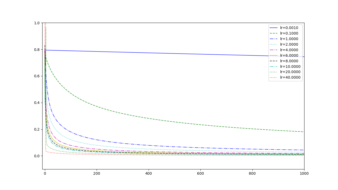
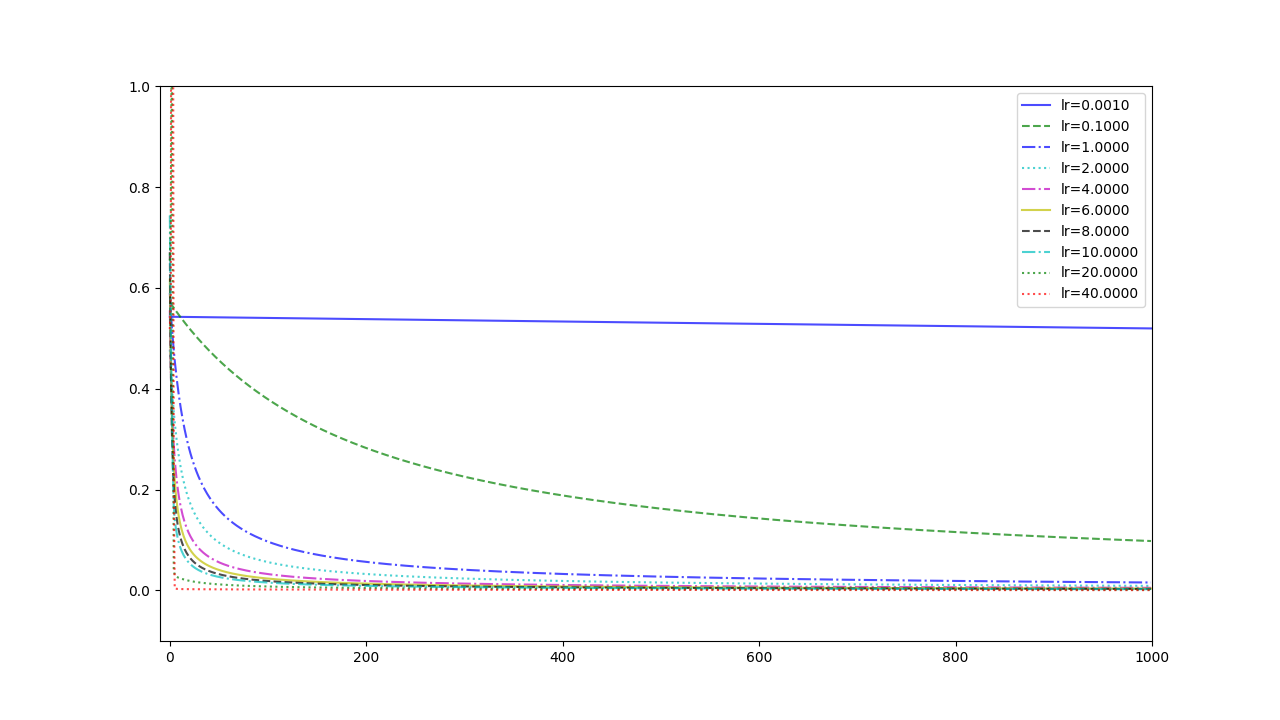
Two hyperparameters are the learning rate and the stop condition. When the error is lower than the stopping threshold, the algorithm stops.

Experiment 1

with the learning rate 1, and different learning rates lead to different convergence rates:

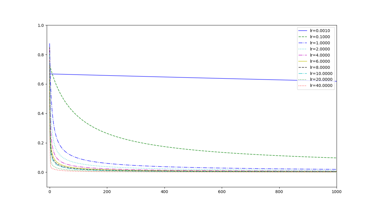
Experiment 2

with the learning rate 1, and different learning rates lead to different convergence rates:

Experiment 3

with the learning rate 1, and different learning rates lead to different convergence rates:

Several Traps in Logistic Regression

1. Input value should be normalized and centered at 0
2. Learning rate is chosen corroding to equation (14) but not \(-\sum_{i=1}^N(t_i-y_i)\mathbf{x}\) because the uncertain coefficient \(N\)
3. parameter vector \(\mathbf{w}\) identifies the direction, so its margin can be arbitrarily large. And to a large \(\mathbf{w}\) , \(y_i(\mathbf{x})\) is very close to \(1\) or \(0\), but it can never be \(1\) or \(0\). So there is no optimization position, and the equation(13) can never be \(0\) which means the algorithm can never stop by himself.
4. The more large margin, more steppen the curve
   • Considering \(\frac{1}{1+e^{-\mathbf{w}^T\mathbf{x}}}\), when the margin of \(\mathbf{w}\) grows, we can write it in a combination of margin \(M\) and direction vector \(\mathbf{w}_d\): \(\frac{1}{1+e^{-M(\mathbf{w_d}^T\mathbf{x}})}\). And the function \(\frac{1}{1+e^{-M(x)}}\) varies according \(M\) is like(when \(M\) grows the logistic function is more like Heaviside step function):

References

Bishop, Christopher M. Pattern recognition and machine learning. springer, 2006.↩︎