Least Squares in Classification

Preliminaries

1. A Simple Linear Regression
2. Least Squares Estimation
3. From Linear Regression to Linear Classification
4. pseudo-inverse

Least Squares for Classification¹

Least-squares for linear regression had been talked about in ‘Simple Linear Regression’. And in this post, we want to find out whether this powerful algorithm can be used in classification.

Recalling the distinction between the properties of classification and regression, two points need to be emphasized again(‘From Linear Regression to Linear Classification’):

1. the targets of regression are continuous but the targets of classification are discrete.
2. the output of the classification hypothesis could be \(\mathbb{P}(\mathcal{C}_k|\mathbf{x})\) generatively or the output is just a class label \(\mathcal{C}_k\) discriminatively.

The generative model will be talked about in other posts. And we focus on discriminative models in these posts which means our hypothesis directly gives which class the input belongs to.

We want to use least-squares methods which had been designed and proved for linear regression. And what we could do to extend the least-squares method to classification are:

1. modifying the type of output and
2. designing a discriminative model

Modifying the type of output is to convert the class label into a number, like ‘apple’ to \(1\), ‘orange’ to 0. And when we use the 1-of-K label scheme(https://anthony-tan.com/From-Linear-Regression-to-Linear-Classification/), we could build the model with \(K\) linear functions:

\[ \begin{aligned} y_1(\mathbf{x})&=\mathbf{w}^T_1\mathbf{x}\\ y_2(\mathbf{x})&=\mathbf{w}^T_2\mathbf{x}\\ \vdots&\\ y_K(\mathbf{x})&=\mathbf{w}^T_K\mathbf{x}\\ \end{aligned}\tag{1} \]

where \(\mathbf{x}=\begin{bmatrix}1&x_1&x_2&\cdots&x_n\end{bmatrix}^T\) and \(\mathbf{w}_i=\begin{bmatrix}w_0&w_1&w_2&\cdots&w_n\end{bmatrix}^T\) for \(i=1,2,\cdots,K\). And \(y_i\) is the \(i\) th component of 1-of-K output for \(i=1,2,\cdots,K\). Clearly, the output of each \(y_i(\mathbf{x})\) is continuous and could not be just \(0\) or \(1\). So we set the largest value to be 1 and others 0.

We had discussed the linear regression with the least squares in a ‘single-target’ regression problem. And that idea can also be employed in the multiple targets regression. And these \(K\) parameter vectors \(\mathbf{w}_i\) can be calculated simultaneously. We can rewrite the equation (1) into the matrix form:

\[ \mathbf{y}(\mathbf{x})=W^T\mathbf{x}\tag{2} \]

where the \(i\)th column of \(W\) is \(\mathbf{w}_i\)

Then we employ the least square method for a sample:

\[ \{(\mathbf{x}_1,\mathbf{t}_1),(\mathbf{x}_2,\mathbf{t}_2),\cdots,(\mathbf{x}_m,\mathbf{t}_m)\} \tag{3} \]

where \(\mathbf{t}\) is a \(K\)-dimensional target consisting of \(k-1\) 0’s and one ‘1’. And each diminsion of output \(\mathbf{y}(\mathbf{x})_i\) is the regression result of the corresponding dimension of target \(t_i\). And we build up the input matrix \(X\) of all \(m\) input consisting of \(\mathbf{x}^T\) as rows:

\[ X=\begin{bmatrix} -&\mathbf{x}^T_1&-\\ -&\mathbf{x}^T_2&-\\ &\vdots&\\ -&\mathbf{x}^T_K&- \end{bmatrix}\tag{4} \]

The sum of square errors is:

\[ E(W)=\frac{1}{2}\mathrm{Tr}\{(XW-T)^T(XW-T)\} \tag{5} \]

where the matrix \(T\) is the target matrix whose \(i\) th row in target vevtor \(\mathbf{t}^T_i\). The trace operation is employed because the only the value \((W\mathbf{x}^T_i-\mathbf{t}_i)^T(W\mathbf{x}_i^T-\mathbf{t}_i)\) for \(i=1,2,\cdots,m\) is meaningful, but \((W\mathbf{x}^T_i-\mathbf{t}_i)^T(W\mathbf{x}_j^T-\mathbf{t}_j)\) where \(i\neq j\) and \(i,j = 1,2,\cdots,m\) is useless.

To minimize the linear equation in equation(5), we can get its derivative

\[ \begin{aligned} \frac{dE(W)}{dW}&=\frac{d}{dW}(\frac{1}{2}\mathrm{Tr}\{(XW-T)^T(XW-T)\})\\ &=\frac{1}{2}\frac{d}{dW}(\mathrm{Tr}\{W^TX^TXW-T^TXW-W^TX^TT+T^TT\})\\ &=\frac{1}{2}\frac{d}{dW}(\mathrm{Tr}\{W^TX^TXW\}-\mathrm{Tr}\{T^TXW\}\\ &-\mathrm{Tr}\{W^TX^TT\}+\mathrm{Tr}\{T^TT\})\\ &=\frac{1}{2}\frac{d}{dW}(\mathrm{Tr}\{W^TX^TXW\}-2\mathrm{Tr}\{T^TXW\}+\mathrm{Tr}\{T^TT\})\\ &=\frac{1}{2}(X^TXW-X^TT) \end{aligned}\tag{6} \]

and set it equal to \(\mathbf{0}\):

\[ \begin{aligned} \frac{1}{2}(X^TXW-X^TT )&= \mathbf{0}\\ W&=(X^TX)^{-1}X^TT \end{aligned}\tag{7} \]

where we assume \(X^TX\) can be inverted. The component \((X^TX)^{-1}X^T\) is also called pseudo-inverse of the matrix \(X\) and it is always denoted as \(X^{\dagger}\).

Code and Result

The code of this algorithm is relatively simple because we have programmed the linear regression before which has the same form of equation (7).

What we should care about is the formation of these matrices \(W\), \(X\), and \(T\).

we should first convert the target value into the 1-of-K form:

def label_convert(y, method ='1-of-K'):
    if method == '1-of-K':
        label_dict = {}
        number_of_label = 0
        for i in y:
            if i not in label_dict:
                label_dict[i] = number_of_label
                number_of_label += 1
        y_ = np.zeros([len(y),number_of_label])
        for i in range(len(y)):
            y_[i][label_dict[y[i]]] = 1
        return y_,number_of_label

what we do is count the total number of labels(\(K\))and we set the \(i\) th component of the 1-of-K target to 1 and other components to 0.

The kernel of the algorithm is:

class LinearClassifier():
    def least_square(self, x, y):
        x = np.array(x)
        x_dim = x.shape[0]
        x = np.c_[np.ones(x_dim), x]
        w = np.linalg.pinv(x.transpose().dot(x)).dot(x.transpose()).dot(y)
        return w.transpose()

the line x = np.c_[np.ones(x_dim), x] is to augment the input vector \(\mathbf{x}\) with a dummy value \(1\). And the transpose of the result is to make each row represent a weight vector of eqation (2). The entire project can be found The entire project can be found https://github.com/Tony-Tan/ML and please star me 🥰.

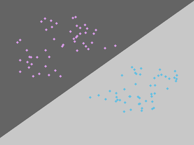
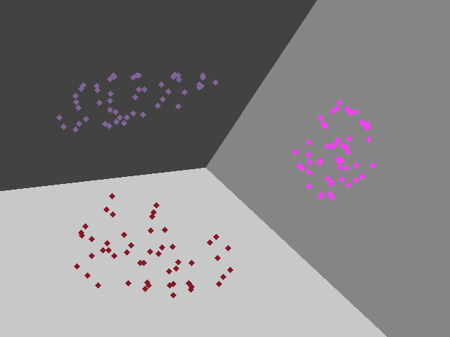
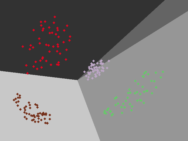
I have tested the algorithm in several training sets, and the result is like the following figures:

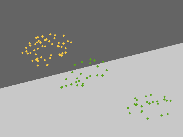
Problems of Least Squares

1. Lack of robustness if outliers (Figure 2 illustrates this problem)
2. Sum of squares error penalizes the predictions that are too correct(the decision boundary will be tracked to the outlinear as the points at right bottom corner in figure 2)
3. Least-squares workes for regression when we assume the target data has a Gaussian distribution and then the least-squares method maximizes the likelihood function. The distribution of targets in these classification tasks is not Gaussian.

References

Bishop, Christopher M. Pattern recognition and machine learning. springer, 2006.↩︎