Priliminaries
- A Simple Linear Regression
- the column space
Another Example of Linear Regression 1
In the blog A Simple Linear Regression, squares of the difference between the output of a predictor and the target were used as a loss function in a regression problem. And it could be also written as:
\[ \ell(\hat{\mathbf{y}}_i,\mathbf{y}_i)=(\hat{\mathbf{y}}_i-\mathbf{y}_i)^T(\hat{\mathbf{y}}_i-\mathbf{y}_i) \tag{1} \]
The linear regression model in a matrix form is:
\[ y=\mathbf{w}^T\mathbf{x}+\mathbf{b}\tag{2} \]
What we do in this post is analyze the least-squares methods from two different viewpoints
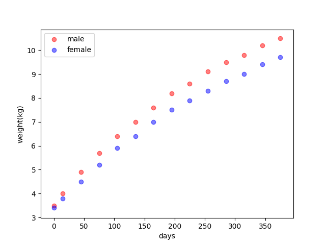
Consider a new training set, newborn weights, and time from the WHO:
| Day | Male(kg) | Female(kg) |
|---|---|---|
| 0 | 3.5 | 3.4 |
| 15 | 4.0 | 3.8 |
| 45 | 4.9 | 4.5 |
| 75 | 5.7 | 5.2 |
| 105 | 6.4 | 5.9 |
| 135 | 7.0 | 6.4 |
| 165 | 7.6 | 7.0 |
| 195 | 8.2 | 7.5 |
| 225 | 8.6 | 7.9 |
| 255 | 9.1 | 8.3 |
| 285 | 9.5 | 8.7 |
| 315 | 9.8 | 9.0 |
| 345 | 10.2 | 9.4 |
| 375 | 10.5 | 9.7 |
View of algebra
This is just what the post A Simple Linear Regression did. The core idea of this view is that the loss function is quadratic so its stationary point is the minimum or maximum. Then what to do is just find the stationary point.
And its result is: 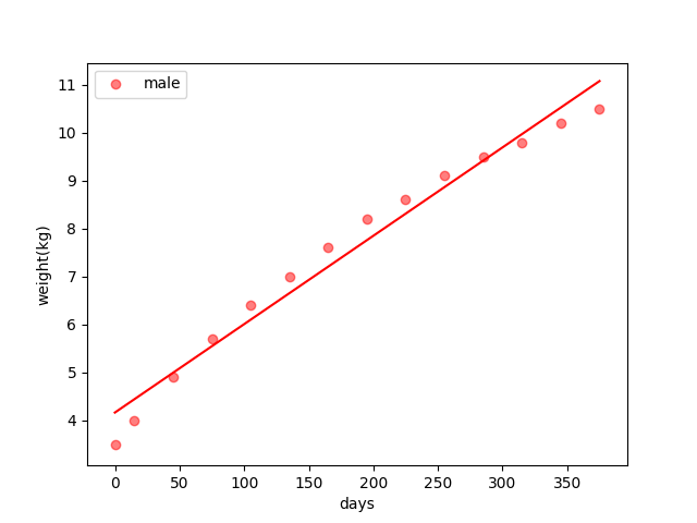
View of Geometric
Such a simple example with just two parameters above had almost messed us up in calculation. However, the practical task may have more parameters, say hundreds or thousands of parameters. It is impossible for us to solve that in a calculus way.
Now let’s review the linear relation in equation (2) and when we have a training set of \(m\) points : \[ \{(\mathbf{x}_1,y_1),(\mathbf{x}_2,y_2),\dots,(\mathbf{x}_m,y_m)\}\tag{3} \]
Because they are sampled from an identity “machine”. They can be stacked together in a matrix form as:
\[ \begin{bmatrix} y_1\\ y_2\\ \vdots\\ y_m \end{bmatrix}=\begin{bmatrix} -&\mathbf{x}_1^T&-\\ -&\mathbf{x}_2^T&-\\ &\vdots&\\ -&\mathbf{x}_m^T&- \end{bmatrix}\mathbf{w}+I_m\mathbf{b}\tag{4} \]
where \(I_m\) is an identical matrix whose column and row is \(m\) and \(\mathbf{b}\) is \(b\) repeating \(m\) times. To make the equation shorter and easier to calculate, we can put \(b\) into the vector \(\mathbf{w}\) like:
\[ \begin{bmatrix} y_1\\ y_2\\ \vdots\\ y_m \end{bmatrix}=\begin{bmatrix} 1&-&\mathbf{x}_1^T&-\\ 1&-&\mathbf{x}_2^T&-\\ 1&&\vdots&\\ 1&-&\mathbf{x}_m^T&- \end{bmatrix} \begin{bmatrix} b\\ \mathbf{w} \end{bmatrix} \tag{5} \]
We use a simplified equation to represent the relation in equation(5): \[ \mathbf{y} = X\mathbf{w}\tag{6} \]
From the linear algebra points, equation(6) represents that \(\mathbf{y}\) is in the column space of \(X\). However, when \(\mathbf{y}\) isn’t, the equation (6) does not hold anymore. And what we need to do next is to find a vector \(\mathbf{\hat{y}}\) in the column space which is the closest one to the vector \(\mathbf{y}\):
\[ \arg\min_{\mathbf{\hat{y}}=X\mathbf{w}} ||\mathbf{y}-\mathbf{\hat{y}}||\tag{7} \]
And as we have known, the projection of \(\mathbf{y}\) to the column space of \(X\) has the shortest distance to \(\mathbf{y}\)
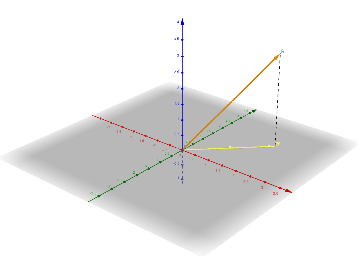
According to linear algebra, the closest vector in a subspace to a vector is its projection in that subspace. Then our mission now is to find \(\mathbf{w}\) to make:
\[ \mathbf{\hat{y}} = X\mathbf{w}\tag{8} \]
where \(\mathbf{\hat{y}}\) is the projection of \(\mathbf{y}\) in the column space of \(X\).
According to the projection equation in linear algebra:
\[ \mathbf{\hat{y}}=X(X^TX)^{-1}X^T\mathbf{y}\tag{22} \]
Then substitute equation (8) into equation (9) and assuming \((X^TX)^{-1}\) exists:
\[ \begin{aligned} X\mathbf{w}&=X(X^TX)^{-1}X^T\mathbf{y}\\ X^TX\mathbf{w}&=X^TX(X^TX)^{-1}X^T\mathbf{y}\\ X^TX\mathbf{w}&=X^T\mathbf{y}\\ \mathbf{w}&=(X^TX)^{-1}X^T\mathbf{y} \end{aligned}\tag{10} \]
To a thin and tall matrix, \(X\), which means that the number of sample points in the training set is far more than the dimension of a sample point, \((X^TX)^{-1}\) exists usually.
Code of Linear Regression(Matrix Form)
import pandas as pds
import numpy as np
import matplotlib.pyplot as plt


class LeastSquaresEstimation():
    def __init__(self, method='OLS'):
        self.method = method

    def fit(self, x, y):
        x = np.array(x).reshape(-1, 1)
        # add a column which is all 1s to calculate bias of linear function
        x = np.c_[np.ones(x.size).reshape(-1, 1), x]
        y = np.array(y).reshape(-1, 1)
        if self.method == 'OLS':
            w = np.linalg.inv(x.transpose().dot(x)).dot(x.transpose()).dot(y)
            b = w[0][0]
            w = w[1][0]
            return w, b


if __name__ == '__main__':
    data_file = pds.read_csv('./data/babys_weights_by_months.csv')
    lse = LeastSquaresEstimation()
    weight_male, bias_male = lse.fit(data_file['day'],data_file['male'])
    day_0 = data_file['day'][0]
    day_end = list(data_file['day'])[-1]
    days = np.array([day_0,day_end])
    plt.scatter(data_file['day'], data_file['male'], c='r', label='male', alpha=0.5)
    plt.scatter(data_file['day'], data_file['female'], c='b', label='female', alpha=0.5)
    plt.xlabel('days')
    plt.ylabel('weight(kg)')
    plt.legend()
    plt.show()
the entire project can be found at https://github.com/Tony-Tan/ML and please star me 😀.
Its output is also like:

Reference
Bishop, Christopher M. Pattern recognition and machine learning. springer, 2006.↩︎