Preliminaries
Learning Rules1
We have built some neural network models in the post ‘An Introduction to Neural Networks’ and as we know architectures and learning rules are two main aspects of designing a useful network. The architectures we have introduced could not be used yet. What we are going to do is to investigate the learning rules for different architectures.
The learning rule is a procedure to modify weights, bias, and other parameters in the model to perform a certain task. There are generally 3 types of learning rules:
- Supervised Learning
- There is a training set of the model that contains a number of input data as well as correct output values that are also known as targets, like the set \(\{\mathbf{p}_1,t_1\},\{\mathbf{p}_2,t_2\},\cdots,\{\mathbf{p}_Q,t_Q\},\) where \(\mathbf{p}_i\) (for \(i<Q\)) is the input of the model and \(t_i\)(for \(i<Q\)) is the corresponding target(any kind of output, like labels, regression values)
- the whole process is:
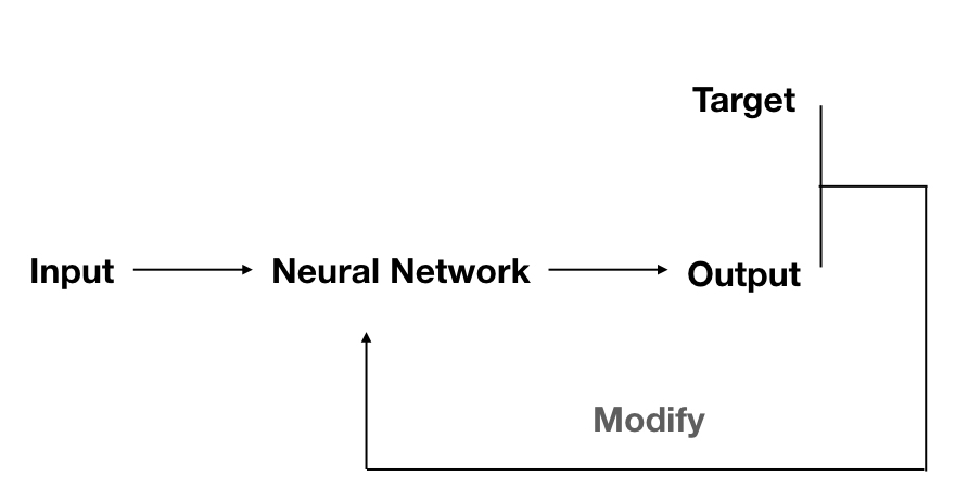
- where target and current output are used to modify the neuron network to produce an output as close to the target as possible according to the input.
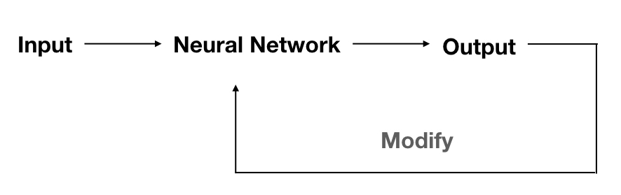
- Unsupervised Learning
- Unlike supervised learning, unsupervised learning doesn’t know the correct output at all, in other words, what the neuron network knows is only the inputs, and how to modify the parameters in the model is depend only on the inputs. This kind of learning is always used to perform clustering operations or vector quantization.
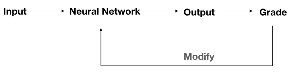
- Reinforcement learning
- it is another learning rule which is more like supervised learning and works more like a biological brain.
- there is no correct target as well but there is a grade to measure the performance of the network over some sequence of input.
Perceptron Architecture
A perceptron is an easy model of a neuron, and what we are interested in is how to design a learning rule or develop a certain algorithm to make a perceptron possible to classify input signals. Perceptron is the easiest neuron model, and it is a good basis for more complex networks.
In a perceptron, it has weights, biases, and transfer functions. These are basic components of a neuron model. However, the transfer function here is specialized as a ‘hard limit function’
\[ f(x) = \begin{cases} 0& \text{ if } x<0\\ 1& \text{ if } x\geq 0 \end{cases}\tag{1} \]
and abbreviated notation with a layer of \(S\) neuron network is:
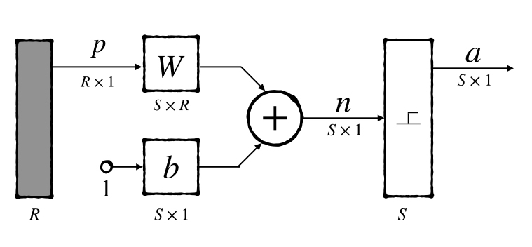
where \(W\) are the weight matrix of \(S\) perceptrons. And each row of the matrix contains all the weight of a perceptron.
Single-Neuron Perceptron
In some simple models, we can visualize a line or a plane named ‘decision boundary’ which is determined by the input vectors who make the input of its transfer function \(n=0\). For instance, in a 2-dimensional linear classification task, we were asked to find a line that can separate the input points into two different classes. This line here acts as a decision boundary and all the points on the line would produce \(0\) output through the linear model.
Let’s start to study with one perceptron.
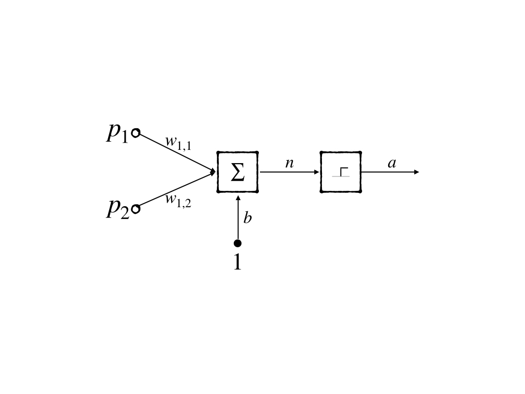
Its decision boundary is the line:
\[ n=w_{1,1}p_1+w_{1,2}p_2+b=0\tag{2} \]
For example, when \(w_{1,1}=1\), \(w_{1,2}=1\) and \(b=-1\), we get the decision boundary:
\[ p_1+p_2-1=0\tag{3} \]
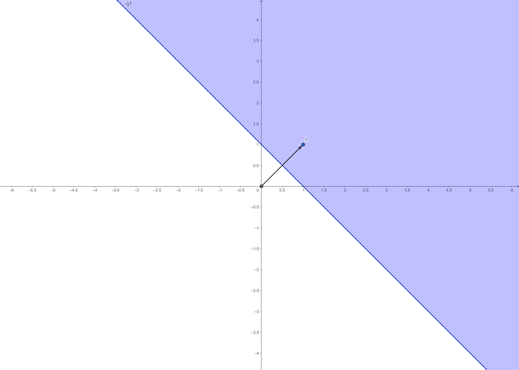
from the figure, we can conclude the weight vector has the following properties:
- \(W\) always points to the purple region where \(n=w_{1,1}p_1+w_{1,2}p_2+b>0\)
- The relation of \(W\) and the direction of the decision boundary is orthogonality.
Can this simple example perform some task? Of course. If we test the input \(\mathbf{p}_1=\begin{bmatrix}0&0\end{bmatrix}^T,\mathbf{p}_1=\begin{bmatrix}0&1\end{bmatrix}^T,\mathbf{p}_1=\begin{bmatrix}1&0\end{bmatrix}^T,\mathbf{p}_1=\begin{bmatrix}1&1\end{bmatrix}^T\) respectively, we could get \(a_1=0,a_2=0,a_3=0,a_4=1\). This is the ‘and’ operation in logical calculation.
| input | output | |
|---|---|---|
| \(\begin{bmatrix}0&0\end{bmatrix}^T\) | \(0\) | |
| \(\begin{bmatrix}0&1\end{bmatrix}^T\) | \(0\) | |
| \(\begin{bmatrix}1&0\end{bmatrix}^T\) | \(0\) | |
| \(\begin{bmatrix}1&1\end{bmatrix}^T\) | \(1\) |
Multiple-Neuron Perceptron
A multiple neuron perceptron is just a combination of some perceptrons, whose weight matrix \(W\) has multiple rows. And the transpose of row \(i\) of the \(W\) is notated as \(_iW\)(column form of the \(i\)th row in \(W\)) then the \(i\) th neuron has the decision boundary:
\[ _iW^T\mathbf{p}+b_i=0\tag{4} \]
For the property of hard limit function that the output could just be one of \(\{0,1\}\). And for \(S\) neurons, there are at most \(2^S\) categories, that is to say to a \(S\) neuron perceptron in one layer it is impossible to solve the problems containing more than \(2^S\) classes.
Perceptron Learning Rule
Perceptron learning rule here is a kind of supervised learning rule. Recall some results above: 1. supervised learning had both input and corresponding correct target. 2. target, the output produced by the current model, and input produced the information on how to modify the model 3. \(W\) always points to the region where the output is \(a=1\)
Constructing Learning Rules
With the above results we try to design the rule and assume training dates are:
\[ \{\begin{bmatrix}1\\2\end{bmatrix},1\},\{\begin{bmatrix}-1\\2\end{bmatrix},0\},\{\begin{bmatrix}0\\-1\end{bmatrix},0\}\tag{5} \]
Assigning Some Initial Values
To modify the model, we need the output which is produced by the weights and input. And for this supervised learning algorithm we have both input and correct outputs (targets), what we need to do is just assign some values to weights(here we omit the bias). Like:
\[ _1W=\begin{bmatrix}1.0\\-0.8\end{bmatrix}\tag{6} \]
Calculating output
The output is easy to be calculated: \[ a=f(_1W^T\mathbf{p}_1)\tag{7} \]
when \(\mathbf{p}_1=\begin{bmatrix}1\\ 2\end{bmatrix}\), we have:
\[ n=\begin{bmatrix}1.0 &-0.8\end{bmatrix}\begin{bmatrix}1\\2\end{bmatrix}=-0.6\\ a=f(-0.6)=0\tag{8} \]
however, the target is \(1\) so this is a wrong prediction of the current model. What we would do is modify the model.
As we mentioned above, \(_1W\) points to the purple region
where the output is \(1\). So we should modify the direction of \(_1W\) close to the direction of \(p_1\).
The intuitive strategy is setting \(_1W=p_i\) when the output is \(0\) while the target is \(1\) and setting \(_1W=-p_i\) when the output is \(1\) while the target is \(0\)(where \(i\) less than the size of the training set). However, there are only three training points in this example, so there are only three possible decision boundaries, it can not guarantee that there must be a line \(_1W=p_i\) that separates the input data correctly.
Although this strategy does not work, it has a good inspiration: 1. if \(t=1\) and \(a=0\), modify \(_1W\) close to \(p_i\) 2. if \(t=0\) and \(a=1\), modify \(_1W\) away from \(p_i\) or modify \(_1W\) close to \(-p_i\) equally 3. if \(t=a\) do nothing
Then we find that the summation of two vectors is closer to each of the two vectors. Then our algorithm becomes:
- if \(t=1\) and \(a=0\), \(_1W^{\text{new}}= _1W^{\text{old}}+p_i\)
- if \(t=0\) and \(a=1\), \(_1W^{\text{new}}= _1W^{\text{old}}-p_i\)
- if \(t=a\) do nothing
Unified Learning Rule
The target and output product information together to modify the model. Here we introduce the most simple but useful information - ‘error’:
\[ e_i=t_i-a_i\tag{9} \]
so, our algorithm is
- if \(t=1\) and \(a=0\) where \(e=1-0=1\): \(_1W^{\text{new}}= _1W^{\text{old}}+p_i\)
- if \(t=0\) and \(a=1\) where \(e=0-1=-1\): \(_1W^{\text{new}}= _1W^{\text{old}}-p_i\)
- if \(t=a\) where \(e=t-a=0\): do nothing
and it’s not hard to notice that \(e\) has the same sign with \(p_i\). Then the algorithm can be simplified as:
\[ _1W^{\text{new}}=_1W^{\text{old}}+e\cdot p_i=_1W^{\text{old}}+(t_i-a_i)\cdot p_i\tag{10} \]
This can be easily extended to bias:
\[ b^{\text{new}}=b^{\text{old}}+e\cdot 1=b^{\text{old}}+(t_i-a_i)\tag{11} \]
and to the multiple neurons perceptron networks, the algorithm in matrix form is:
\[ W^{\text{new}}=W^{\text{old}}+\mathbf{e}\cdot \mathbf{p_i}\\ \mathbf{b}^{\text{new}}=\mathbf{b}^{\text{old}}+\mathbf{e}_i\cdot \mathbf{1}\tag{12} \]
Conclusion
- Perceptron is still working today
- The learning rule of the perceptron is a good example of having a close look at the learning rules of neuron networks
- Perceptron has some connection with other machine learning algorithms like linear classification
- A single perceptron has a lot of limits but multiple layers of perceptrons are more powerful
References
Demuth, H.B., Beale, M.H., De Jess, O. and Hagan, M.T., 2014. Neural network design. Martin Hagan.↩︎