K-means Clustering

Preliminaries

1. Numerical Optimization
   • necessary conditions for maximum
2. K-means algorithm
3. Fisher Linear Discriminant

Clustering Problem¹

The first thing we should do before introducing the algorithm is to make the task clear. A mathematical form is usually the best way.

Clustering is a kind of unsupervised learning task. So there is no correct or incorrect solution because there is no teacher or target in the task. Clustering is similar to classification during predicting since the output of clustering and classification are discrete. However, during training classifiers, we always have a certain target corresponding to every input. On the contrary, clustering has no target at all, and what we have is only

\[ \{x_1,\cdots, x_N\}\tag{1} \]

where \(x_i\in\Re^D\) for \(i=1,2,\cdots,N\). And our mission is to separate the dataset into \(K\) groups where \(K\) has been given before task

An intuitive strategy of clustering is based on two considerations: 1. the distance between data points in the same group should be as small as possible. 2. the distance between data points in the different groups should be as large as possible.

This is a little like Fisher Linear Discriminant. Based on these two points, some concepts could be formed.

The first one is how to represent a group. We take

\[ \mu_i:i\in\{1,2,\cdots, K\}\tag{2} \]

as the prototype associated with \(i\) th group. A group always contains several points, and a spontaneous idea is using the center of all the points belonging to one group as its prototype. To represent which group \(\mathbf{x}_i\) in equation (1) belongs to, an indicator is necessary, and a 1-of-K coding scheme is used:

\[ r_{nk}\in\{0,1\}\tag{3} \]

for \(k=1,2,\cdots,K\) representing the group number and \(n = 1,2,\cdots,N\) denoting the number of sample point, and where \(r_{nk}=1\) then \(r_{nj}=0\) for all \(j\neq k\).

Objective Function

A loss function is a good way to measure the quantity of our model during both the training and testing stages. And in the clustering task loss function could not be used because we have no idea about what is correct. However, we can build another function that plays the same role as the loss function and it is also the target of what we want to optimize.

According to the two base points above, we build our objective function:

\[ J=\sum_{n=1}^{N}\sum_{k=1}^{K}r_{nk}||\mathbf{x}_n-\mu_k||^2\tag{4} \]

In this objective function, the distance is defined as Euclidean distance(However, other measurements of similarity could also be used). Then the mission is to minimize \(J\) by finding some certain \(\{r_{nk}\}\) and \(\{\mu_k\}\)

K-Means Algorithm

Now, let’s represent the famous K-Means algorithm. The method includes two steps:

1. Minimising \(J\) respect to \(r_{nk}\) keeping \(\mu_k\) fixed
2. Minimising \(J\) respect to \(\mu_k\) keeping \(r_{nk}\) fixed

In the first step, according to equation (4), the objective function is linear of \(r_{nk}\). So there is a close solution. Then we set:

\[ r_{nk}=\begin{cases} 1&\text{ if } k=\arg\min_{j}||x_n-\mu_j||^2\\ 0&\text{otherwise} \end{cases}\tag{5} \]

And in the second step, \(r_{nk}\) is fixed and we minimize objective function \(J\). For it is quadratic, the minimum point is on the stationary point where:

\[ \frac{\partial J}{\partial \mu_k}=-\sum_{n=1}^{N}r_{nk}(x_n-\mu_k)=0\tag{6} \]

and we get:

\[ \mu_k = \frac{\sum_{n=1}^{N}r_{nk}x_n}{\sum_{n=1}^{N}r_{nk}}\tag{7} \]

\(\sum_{n=1}^{N} r_{nk}\) is the total number of points from the sample \(\{x_1,\cdots, x_N\}\) who belong to prototype \(\mu_k\) or group \(k\) at current step. And \(\mu_k\) is just the average of all the points in the group \(k\).

This two-step, which was calculated by equation (5),(7), would repeat until \(r_{nk}\) and \(\mu_k\) not change.

The K-means algorithm guarantees to converge because at every step the objective function \(J\) is reduced. So when there is only one minimum, the global minimum, the algorithm must converge.

Input Data Preprocessing before K-means

Most algorithms need their input data to obey some rules. To the K-means algorithm, we rescale the input data to mean 0 and variance 1. This is always done by

\[ x_n^{(i)} = \frac{x_n^{(i)}- \bar{x}^{(i)}}{\delta^{i}} \]

where \(x_n^{(i)}\) is the \(i\) th component of the \(n\) th data point, and \(x_n\) comes from equation (1), \(\bar{x}^{(i)}\) and \(\delta^{i}\) is the \(i\) th mean and standard deviation repectively

Python code of K-means

class K_Means():
    """
    input data should be normalized: mean 0, variance 1
    """
    def clustering(self, x, K):
        """
        :param x: inputs
        :param K: how many groups
        :return: prototype(center of each group), r_nk, which group k does the n th point belong to
        """
        data_point_dimension = x.shape[1]
        data_point_size = x.shape[0]
        center_matrix = np.zeros((K, data_point_dimension))
        for i in range(len(center_matrix)):
            center_matrix[i] = x[np.random.randint(0, len(x)-1)]

        center_matrix_last_time = np.zeros((K, data_point_dimension))
        cluster_for_each_point = np.zeros(data_point_size, dtype=np.int32)
        # -----------------------------------visualization-----------------------------------
        # the part can be deleted
        center_color = np.random.randint(0,1000, (K, 3))/1000.
        plt.scatter(x[:, 0], x[:, 1], color='green', s=30, marker='o', alpha=0.3)
        for i in range(len(center_matrix)):
            plt.scatter(center_matrix[i][0], center_matrix[i][1],  marker='x', s=65, color=center_color[i])
        plt.show()
        # -----------------------------------------------------------------------------------
        while (center_matrix_last_time-center_matrix).all() != 0:
            # E step
            for i in range(len(x)):
                distance_to_center = np.zeros(K)
                for k in range(K):
                    distance_to_center[k] = (center_matrix[k]-x[i]).dot((center_matrix[k]-x[i]))
                cluster_for_each_point[i] = int(np.argmin(distance_to_center))
            # M step
            number_of_point_in_k = np.zeros(K)
            center_matrix_last_time = center_matrix
            center_matrix = np.zeros((K, data_point_dimension))
            for i in range(len(x)):
                center_matrix[cluster_for_each_point[i]] += x[i]
                number_of_point_in_k[cluster_for_each_point[i]] += 1

            for i in range(len(center_matrix)):
                if number_of_point_in_k[i] != 0:
                    center_matrix[i] /= number_of_point_in_k[i]
            # -----------------------------------visualization-----------------------------------
            # the part can be deleted
            print(center_matrix)
            plt.cla()
            for i in range(len(center_matrix)):
                plt.scatter(center_matrix[i][0], center_matrix[i][1], marker='x', s=65,  color=center_color[i])
            for i in range(len(x)):
                plt.scatter(x[i][0], x[i][1], marker='o',s=30, color=center_color[cluster_for_each_point[i]],alpha=0.7)
            plt.show()
            # -----------------------------------------------------------------------------------
        return center_matrix, cluster_for_each_point

and the entire project can be found : https://github.com/Tony-Tan/ML and please star me(^_^).

Results during K-means

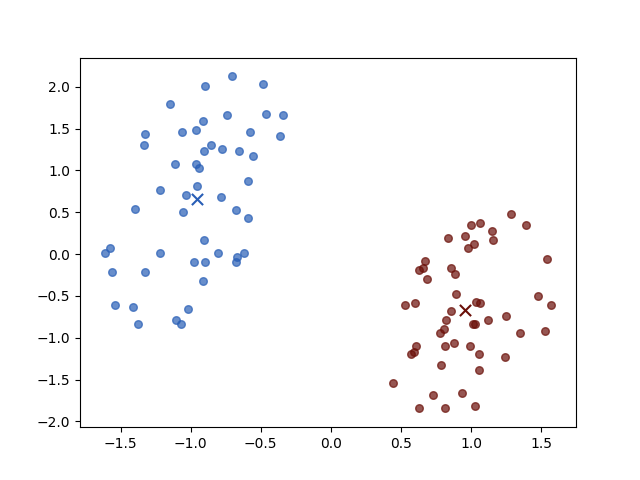
We use a tool https://github.com/Tony-Tan/2DRandomSampleGenerater to generate the input data from:

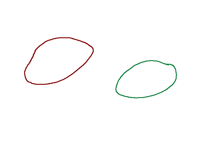
There are two classes the brown circle and the green circle. Then the K-means algorithm initial two prototypes, the centers of groups, randomly:

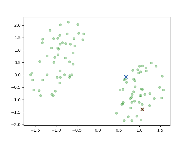
the two crosses represent the initial centers \(\mu_i\). And then we iterate the two steps:

Iteration 1

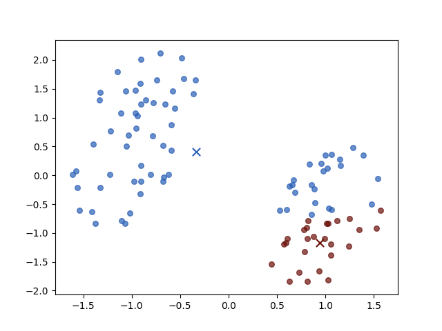
Iteration 2

Iteration 3

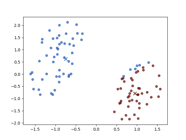
Iteration 4

The result of iterations 3 and 4 do not vary for both objective function value \(J\) and parameters. Then the algorithm stopped.

And different initial centers may have different convergence speeds, but they always have the same stop positions.

References

Bishop, Christopher M. Pattern recognition and machine learning. springer, 2006.↩︎