Implement of Perceptron

Preliminaries

1. An Introduction to Neural Networks
2. Neuron Model and Network Architecture
3. Perceptron Learning Rule

Implement of Perceptron¹

What we need to do next is to implement the algorithm described in ‘Perceptron Learning Rule’ and observe the effect of 1. different parameters, 2. different training sets, 3. and different transfer functions.

A single neuron perceptron consists of a linear combination and a threshold operation simply. So we note its capacity is close to a linear classification. Then our experiments should be done with samples that are linearly separable.

Before our experiments, the first mission that comes to us is to find some or design some training set. That is the data like:

\[ \{(\begin{bmatrix}1\\2\end{bmatrix},1),(\begin{bmatrix}-1\\2\end{bmatrix},0),(\begin{bmatrix}0\\-1\end{bmatrix},0)\} \]

containing inputs(2-dimensional) and corresponding targets. This training set containing 3 points can be generated by hand, but when we need more than 100 points, we need a tool.

Generating of Sample

The tool can be found at https://github.com/Tony-Tan/2DRandomSampleGenerater. And please star it!

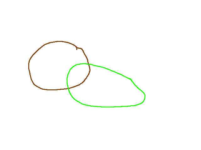
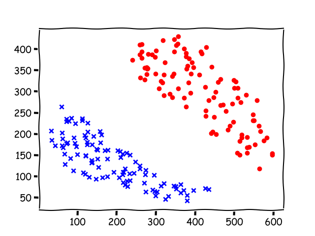
This script used an image as input, and a different color in the image means different classes and the regions should be of the closed forms, like:

An image of two classes is fed into the script. And a ’*.csv’ file will be generated. Part of the file is like this:

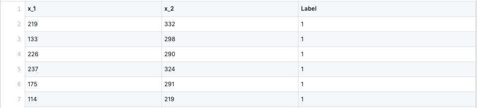
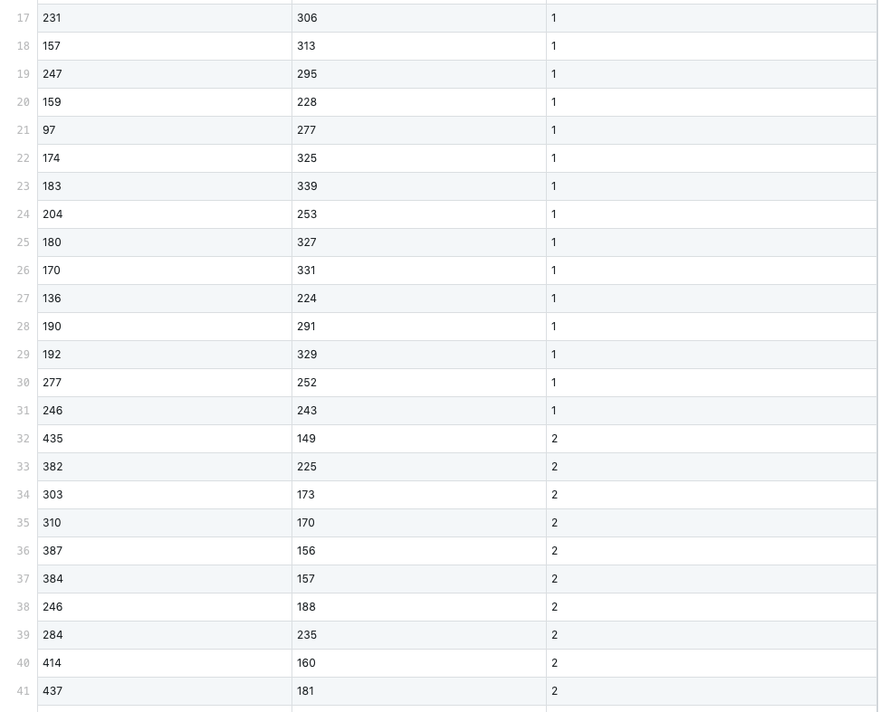
where ‘x_1’ and ‘x_2’ are inputs and ‘Label’ is the target. For the scripts that can generate multi-class training data, the label starts with \(1\) to \(2,3,4,\dots\). So if you want to reassign the target, it should be done in your program.

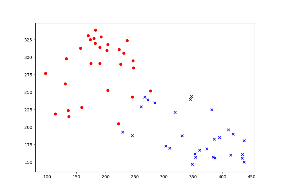
We can also draw a figure of these points and use a different color to identify their classes:

The use of script:

Algorithm and Code

Firstly, we assume we have had a training set that is 2-dimensional linear separable. And our algorithm is:

1. initial weights and bias randomly
2. test inputs one by one,

• if the output is different from the target, go to step 3
• if the whole training set is correctly classified, stop the algorithm.
• else continue to step 2.

3. update \(\mathbf{w}=\mathbf{w}+l\cdot (t-a)\cdot \mathbf{p}\)

• \(\mathbf{w}\) is the weights
• \(\mathbf{p}\) is the input,
• \(t\) is target can be one of \(\{0,1\}\),
• \(a\) is the output, one of \(\{0,1\}\),
• \(l\) is the learning rate, should be \(0< l \leq 1\)

4. update \(b=b+l\cdot (t-a)\cdot 1\)

• \(b\) is the bias
• \(t\) is target can be one of \(\{0,1\}\),
• \(a\) is the output, can be one of \(\{0,1\}\),
• \(l\) is the learning rate, should be \(0< l \leq 1\)

5. go back to 2.

The whole code can be found: https://github.com/Tony-Tan/NeuronNetworks/tree/master/simple_perceptron, and the main part of the code is:

def convergence_algorithm(self, lr=1.0, max_iteration_num = 1000000):
 for epoch in range(max_iteration_num):

 all_inputs_predict_correctly = True
 for x, label in zip(self.X, self.labels):
 predict_value = self.process(x)
 if predict_value == label:
 continue
 else:
 all_inputs_predict_correctly = False
 self.weights += lr*(label - predict_value)* x
 print(str(epoch) + str(' : ') + str(self.weights[0]))

 if all_inputs_predict_correctly:
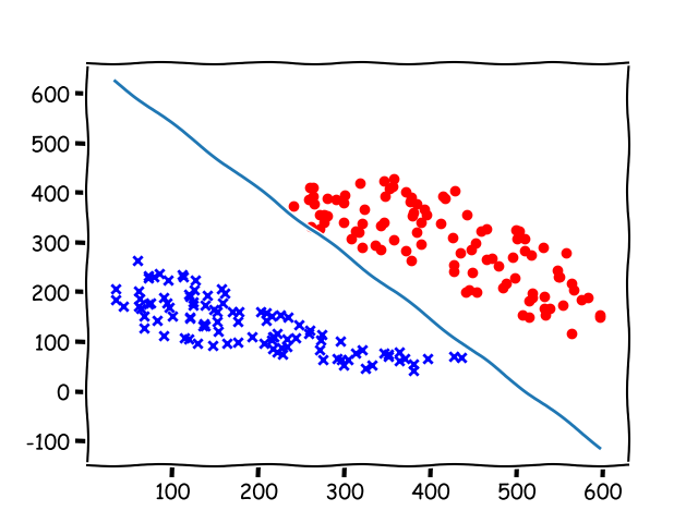
 return True

Training set 4 in the project is shown below.

Training set 4

Points in the training set

Result(after 55449 epochs)

Analysis of the Algorithm

What we are concerned about the algorithm are its precision and efficiency. Because the convergence of the algorithm had been proved, what we are interested in is how to speed up the convergence.

Epoch is a period when every point in the dataset is used once and only once.

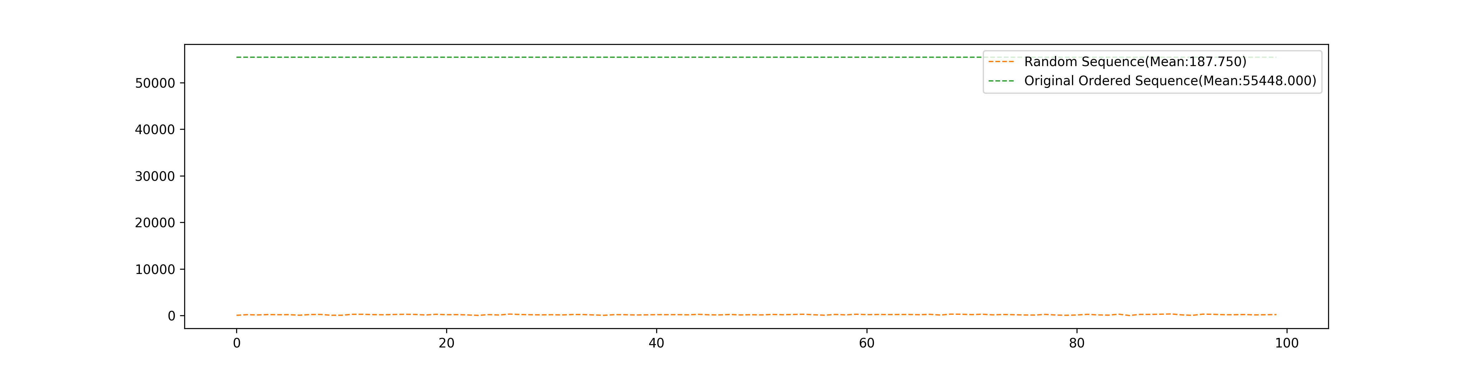
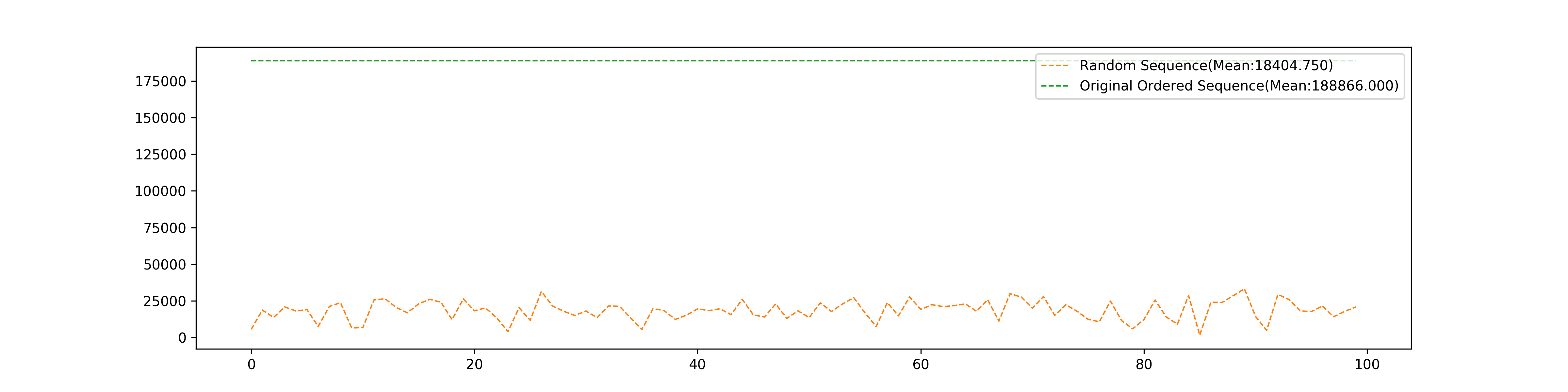
Randomize the input sequence

After 100 times test, we got the number of epochs of random order of the training set used in the algorithm, and the number of epochs of the original order of the training set where the first half part of the dataset belongs to one class, and the last half part belongs to another class"

The following are the result of more training data than above.

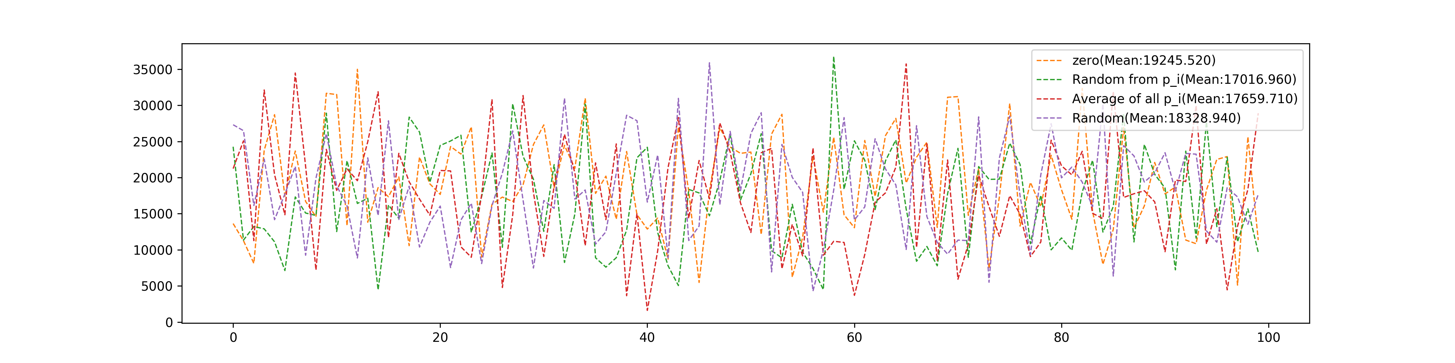
Initial Weights

Weights can be initialed in multiple ways: 1. \(\mathbf{w}=\mathbf{0}\) 2. \(\mathbf{w}=\mathbf{p}_i\), \(\mathbf{p}_i\) is randomly selected from the training set. 3. \(\mathbf{w}=\frac{1}{N}\sum_{i=0}^{N}\mathbf{p}_i\) 4. randomly in (-1000,1000) for every element.

These four different selections’ comparison of epochs they used: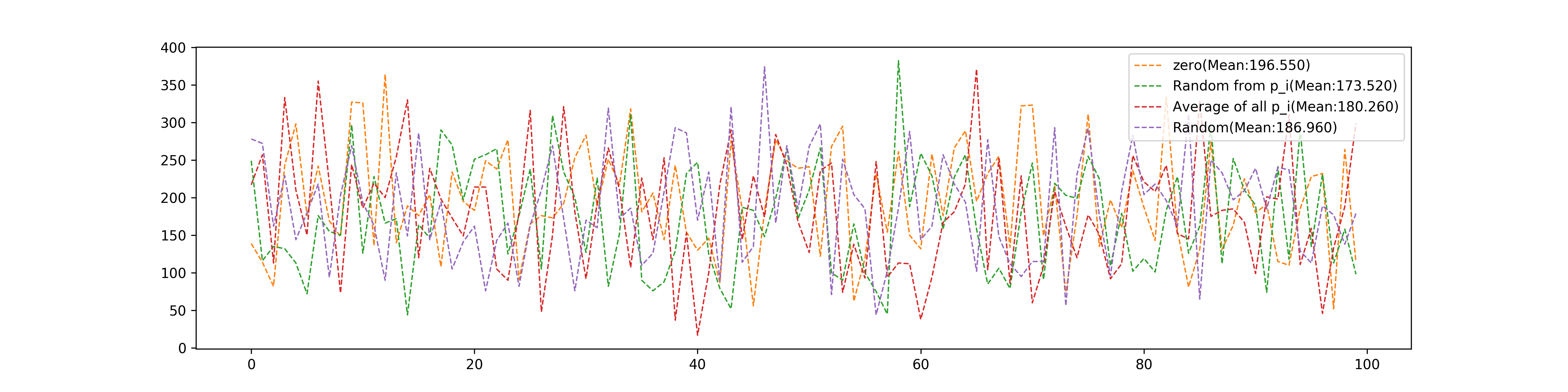

and total modification they used:

Different Transfer Functions

We test: 1. hard limit 2. symmetrical hard limit 3. positive linear 4. hyperbolic tangent sigmoid 5. log sigmoid 6. symmetric saturating linear 7. saturating linear 8. linear

These eight different Transfer Functions’ comparison of epochs they used:

and total modification they used:

Conclusion

1. The random sequence is far better than the original order dataset which distributes different classes of data separately and randomly
2. Initial methods can affect the convergence speed but not too much. Setting weights as one of the input \(p_i\) seems good.
3. The tool to generate samples should be staredhttps://github.com/Tony-Tan/2DRandomSampleGenerater

References

Haykin, Simon. Neural Networks and Learning Machines, 3/E. Pearson Education India, 2010.↩︎