Fisher Linear Discriminant(LDA)

Preliminaries

1. linear algebra

• inner multiplication
• projection

Idea of Fisher linear discriminant¹

‘Least-square method’ in classification can only deal with a small set of tasks. That is because it was designed for the regression task. Then we come to the famous Fisher linear discriminant. This method is also discriminative for it gives directly the class to which the input \(\mathbf{x}\) belongs. Assuming that the linear function

\[ y=\mathbf{w}^T\mathbf{x}+w_0\tag{1} \]

is employed as before. Then the threshold function \(f(\mathbf{y})=\begin{cases}1 &\text{ if } y\leq 0\\0 &\text{ otherwise }\end{cases}\) was employed. If \(y<0\) or equivalenttly \(\mathbf{w}^T\mathbf{x}\leq -w_0\) , \(\mathbf{x}\) belongs to \(\mathcal{C}_1\), or it belongs to \(\mathcal{C}_2\).

This is an intuitive classification framework, but if such kinds of parameters exist and how to find them out is still a hard problem.

From the linear algebra view, when we set \(w_0=0\) the equation (1) can be viewed as the vector \(\mathbf{x}\) projecting on vector \(\mathbf{w}\).

And a good parameter vector direction and a threshold may solve this problem. And the measurement of how good the parameter vector direction is has some different candidates.

Distance Between Class Center

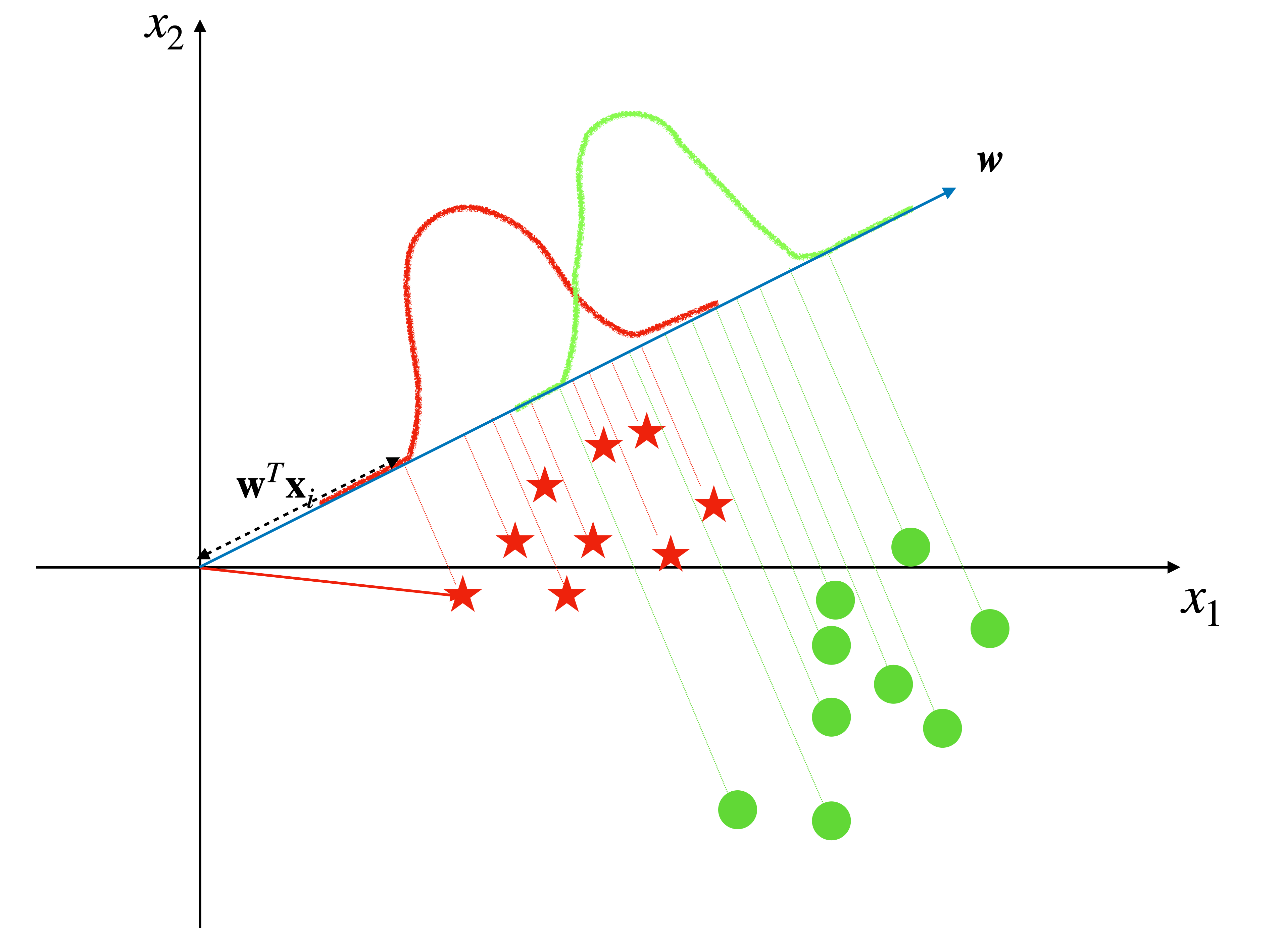
The first strategy that comes to us is to maximize the distance between the projections of the centers of different classes.

The first step is to get the center of a class \(\mathcal{C}_k\) whose size is \(N_k\) by:

\[ \mathbf{m}_k=\frac{1}{N_k}\sum_{x_i\in \mathcal{C}_k}\mathbf{x}_i\tag{2} \]

So the distance between the projections \(m_1\), \(m_2\) of centers of the two classes, \(\mathbf{m}_1\), \(\mathbf{m}_2\) is:

\[ m_1-m_2=\mathbf{w}^T(\mathbf{m}_1-\mathbf{m}_2)\tag{3} \]

And for the \(\mathbf{w}\) here is referred to as the direction vector, its margin is \(1\):

\[ ||\mathbf{w}||=1\tag{4} \]

When \(\mathbf{w}\) has the same direction with \(\mathbf{m}_1-\mathbf{m}_2\), equation(3) get its maximum value.

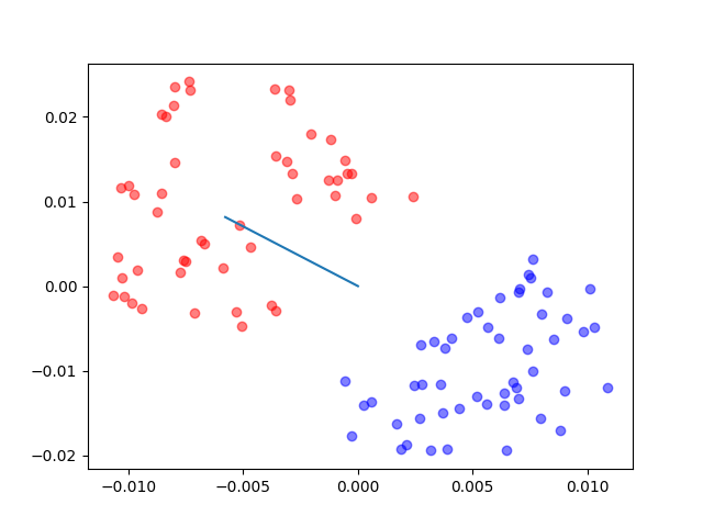
Then the result looks like this:

The blue star and blue circle are the center of red stars and green circles, respectively. and the blue arrow is the direction we want in which the projections of center points have the longest distance.

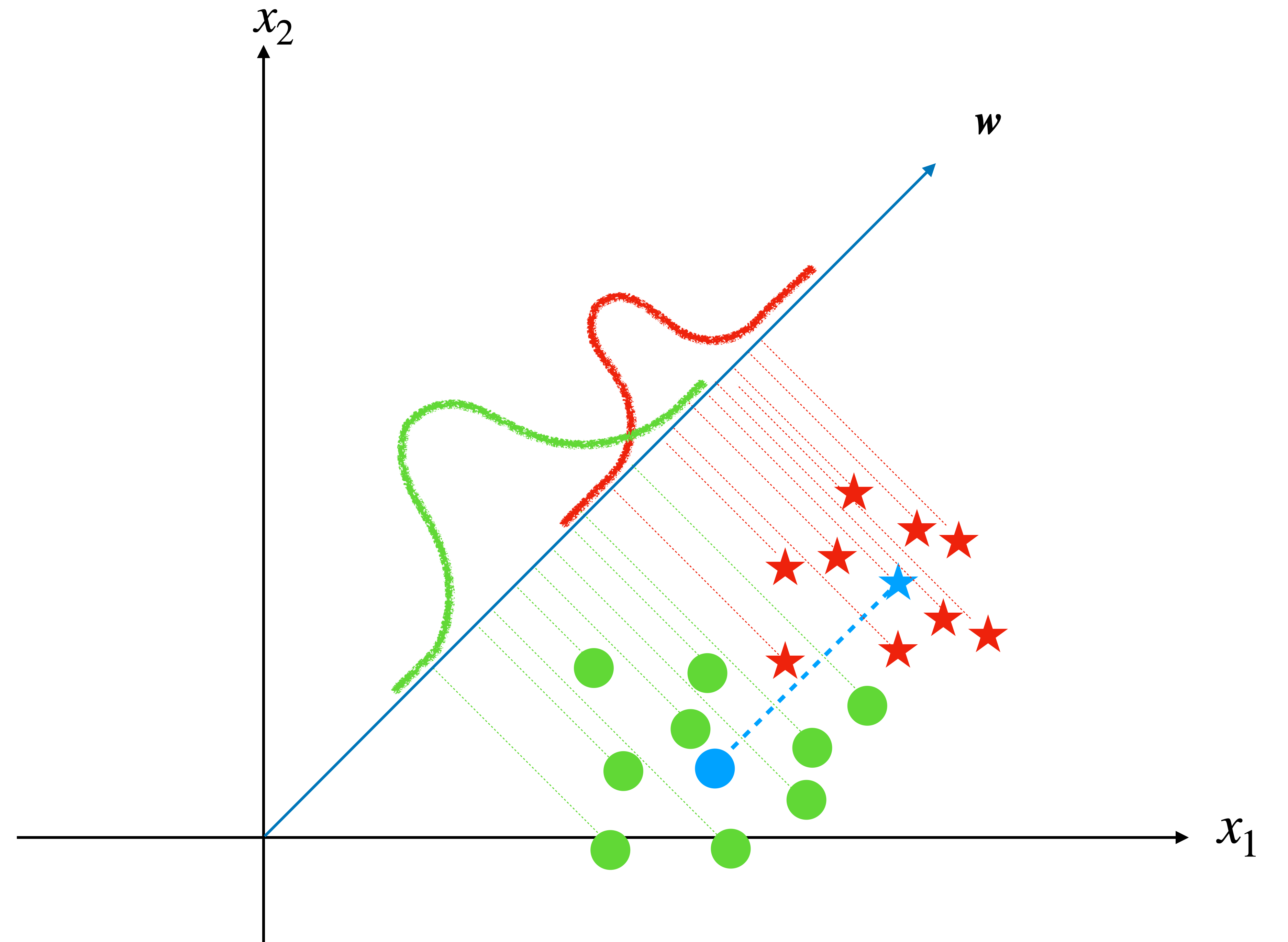
With our observation, this line does not give the optimum solution. Because, although the projections of centers have the longest distance on this line, the projections of all sample points scatter into a relatively large region and some of them from different classes have been mixed up.

This phenomenon exists in our daily life. For example, when two seats are closed, the people sitting on them do not have enough space(this is the original condition). Then we move the seats and make them a little farther from each other(make the projections of centers far from each other). But this time, two big guys come to sit on them(the projection has a big variance), and the space is still not enough.

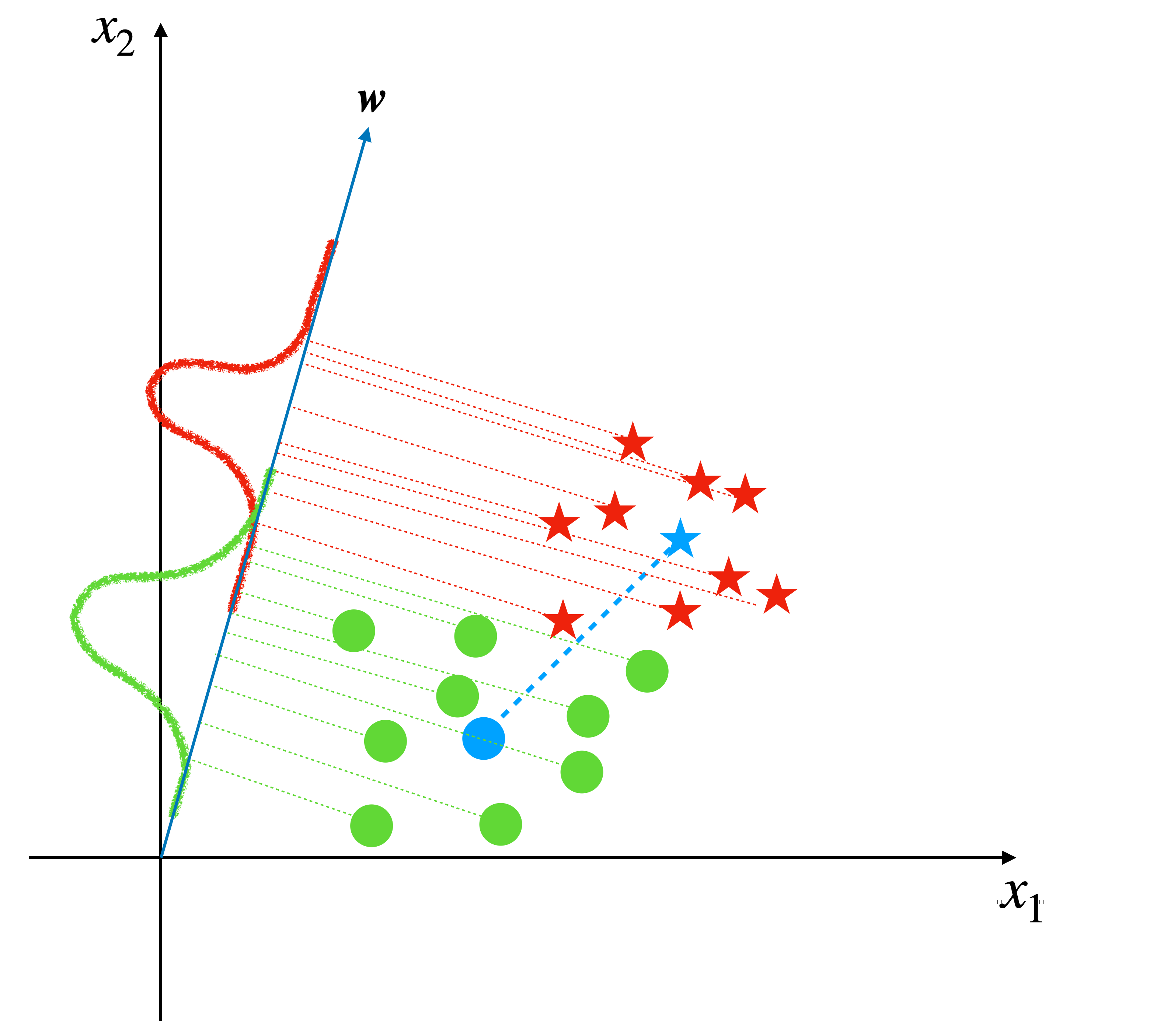
In our problem, the projections of the points of a class are the big guys. We need to make the projection of centers far away from each other and make the projections of points in one class slender (which means a lower variance) at the same time.

The variance of the projected points of class \(k\) can be calculated by:

\[ s^2_k=\sum_{n\in \mathcal{C}_k}(y_n - m_k)^2\tag{5} \]

and it is also called within-class variance.

To make the seat comfortable for people who sit on them, we need to make the seat as far as possible from each other(maximize \((m_2-m_1)^2\)) and only allow children to sit(minimize the sum of within-class variance).

Fisher criterion satisfies this requirement:

\[ J(\mathbf{w})=\frac{(m_2-m_1)^2}{s_1^2+s_2^2}\tag{6} \]

And \(J(\mathbf{w})\) in details is:

\[ \begin{aligned} J(\mathbf{w})&=\frac{(m_2-m_1)^2}{s_1^2+s_2^2}\\ &=\frac{(\mathbf{w}^T(\mathbf{m}_1-\mathbf{m}_2))^T(\mathbf{w}^T(\mathbf{m}_1-\mathbf{m}_2))}{\sum_{n\in \mathcal{C}_1}(y_n - m_1)^2+\sum_{n\in \mathcal{C}_2}(y_n - m_2)^2}\\ &=\frac{(\mathbf{w}^T(\mathbf{m}_1-\mathbf{m}_2))^T(\mathbf{w}^T(\mathbf{m}_1-\mathbf{m}_2))} {\sum_{n\in \mathcal{C}_1}(\mathbf{w}^T\mathbf{x}_n - \mathbf{w}^T\mathbf{m}_1)^2+\sum_{n\in \mathcal{C}_2}(\mathbf{w}^T\mathbf{x}_n - \mathbf{w}^T\mathbf{m}_2)^2}\\ &=\frac{\mathbf{w}^T(\mathbf{m}_1-\mathbf{m}_2)(\mathbf{m}_1-\mathbf{m}_2)^T\mathbf{w}} {\mathbf{w}^T(\sum_{n\in \mathcal{C}_1}(\mathbf{x}_n - \mathbf{m}_1)(\mathbf{x}_n - \mathbf{m}_1)^T+\sum_{n\in \mathcal{C}_2}(\mathbf{x}_n - \mathbf{m}_2)(\mathbf{x}_n - \mathbf{m}_2)^T)\mathbf{w}} \end{aligned}\tag{7} \]

And we can set:

\[ \begin{aligned} S_B &= (\mathbf{m}_1-\mathbf{m}_2)(\mathbf{m}_1-\mathbf{m}_2)^T\\ S_W &= \sum_{n\in \mathcal{C}_1}(\mathbf{x}_n - \mathbf{m}_1)(\mathbf{x}_n - \mathbf{m}_1)^T+\sum_{n\in \mathcal{C}_2}(\mathbf{x}_n - \mathbf{m}_2)(\mathbf{x}_n - \mathbf{m}_2)^T \end{aligned}\tag{8} \]

where \(S_B\) represents the covariance matrix Between classes, and \(S_W\) represents the Within classes covariance. Then the equation(8) becomes:

\[ \begin{aligned} J(\mathbf{w})&=\frac{\mathbf{w}^TS_B\mathbf{w}}{\mathbf{w}^TS_W\mathbf{w}} \end{aligned}\tag{9} \]

To maximise the \(J(\mathbf{w})\), we should differentiat equation (9) with respect to \(\mathbf{w}\) firstly:

\[ \begin{aligned} \frac{\partial }{\partial \mathbf{w}}J(\mathbf{w})&=\frac{\partial }{\partial \mathbf{w}}\frac{\mathbf{w}^TS_B\mathbf{w}}{\mathbf{w}^TS_W\mathbf{w}}\\ &=\frac{(S_B+S_B^T)\mathbf{w}(\mathbf{w}^TS_W\mathbf{w})-(\mathbf{w}^TS_B\mathbf{w})(S_W+S_W^T)\mathbf{w}}{(\mathbf{w}^TS_W\mathbf{w})^T(\mathbf{w}^TS_W\mathbf{w})} \end{aligned}\tag{10} \]

and set it to zero:

\[ \frac{(S_B+S_B^T)\mathbf{w}(\mathbf{w}^TS_W\mathbf{w})-(\mathbf{w}^TS_B\mathbf{w})(S_W+S_W^T)\mathbf{w}}{(\mathbf{w}^TS_W\mathbf{w})^T(\mathbf{w}^TS_W\mathbf{w})}=0\tag{11} \]

and then:

\[ \begin{aligned} (S_B+S_B^T)\mathbf{w}(\mathbf{w}^TS_W\mathbf{w})&=(\mathbf{w}^TS_B\mathbf{w})(S_W+S_W^T)\mathbf{w}\\ (\mathbf{w}^TS_W\mathbf{w})S_B\mathbf{w}&=(\mathbf{w}^TS_B\mathbf{w})S_W\mathbf{w} \end{aligned}\tag{12} \]

Because \((\mathbf{w}^TS_W\mathbf{w})\) and \((\mathbf{w}^TS_B\mathbf{w})\) are scalars and according equation (8) when we multiply both sides by \(\mathbf{w}\) and we have

\[ S_B \mathbf{w}= (\mathbf{m}_1-\mathbf{m}_2)((\mathbf{m}_1-\mathbf{m}_2)^T\mathbf{w})\tag{13} \]

and \((\mathbf{m}_1-\mathbf{m}_2)^T\mathbf{w}\) is a scalar and \(S_B\mathbf{w}\) have the same direction with \((\mathbf{m}_1-\mathbf{m}_2)\)

so the equation (12) can be written as:

\[ \begin{aligned} \mathbf{w}&\propto S^{-1}_WS_B\mathbf{w}\\ \mathbf{w}&\propto S^{-1}_W(\mathbf{m}_1-\mathbf{m}_2) \end{aligned}\tag{14} \]

So, up to now, we have had a result parameter vector \(\mathbf{w}\) based on maximizing Fisher Criterion.

Code

The code of the process is relatively easy:

class LinearClassifier():

    def fisher(self, x, y):
        x = np.array(x)
        x_dim = x.shape[1]
        m_1 = np.zeros(x_dim)
        m_1_size = 0
        m_2 = np.zeros(x_dim)
        m_2_size = 0
        for i in range(len(y)):
            if y[i] == 0:
                m_1 = m_1 + x[i]
                m_1_size += 1
            else:
                m_2 = m_2 + x[i]
                m_2_size += 1
        if m_1_size != 0 and m_2_size != 0:
            m_1 = (m_1/m_1_size).reshape(-1, 1)
            m_2 = (m_2/m_2_size).reshape(-1, 1)
        s_c_1 = np.zeros([x_dim, x_dim])
        s_c_2 = np.zeros([x_dim, x_dim])
        for i in range(len(y)):
            if y[i] == 0:
                s_c_1 += (x[i] - m_1).dot((x[i] - m_1).transpose())
            else:
                s_c_2 += (x[i] - m_2).dot((x[i] - m_2).transpose())
        s_w = s_c_1 + s_c_2

        return np.linalg.inv(s_w).dot(m_2-m_1)

The entire project can be found https://github.com/Tony-Tan/ML and please star me.

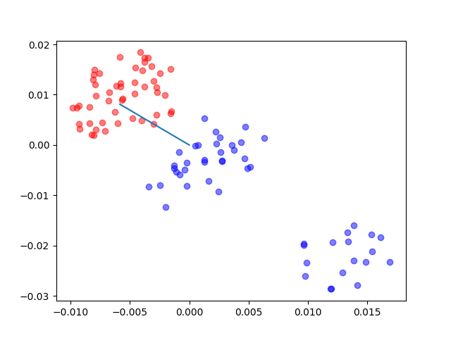
The results of the code(where the line is the one to which the points are projected):

References

Bishop, Christopher M. Pattern recognition and machine learning. springer, 2006. And what we should do is estimate the parameters of the model.↩︎