EM Algorithm

Preliminaries

1. Gaussian distribution
2. log-likelihood
3. Calculus
   • partial derivative
   • Lagrange multiplier

EM Algorithm for Gaussian Mixture¹

Analysis

Maximizing likelihood could not be used in the Gaussian mixture model directly, because of its severe defects which we have come across at ‘Maximum Likelihood of Gaussian Mixtures’. With the inspiration of K-means, a two-step algorithm was developed.

The objective function is the log-likelihood function:

\[ \begin{aligned} \ln \Pr(\mathbf{x}|\mathbf{\pi},\mathbf{\mu},\Sigma)&=\ln (\Pi_{n=1}^N\sum_{j=1}^{K}\pi_k\mathcal{N}(\mathbf{x}|\mathbf{\mu}_k,\Sigma_k))\\ &=\sum_{n=1}^{N}\ln \sum_{j=1}^{K}\pi_j\mathcal{N}(\mathbf{x}_n|\mathbf{\mu}_j,\Sigma_j)\\ \end{aligned}\tag{1} \]

\(\mu_k\)

The condition that must be satisfied at a maximum of log-likelihood is the derivative(partial derivative) of parameters are \(0\). So we should calculate the partial derivatives of \(\mu_k\):

\[ \begin{aligned} \frac{\partial \ln \Pr(X|\pi,\mu,\Sigma)}{\partial \mu_k}&=\sum_{n=1}^N\frac{-\pi_k \mathcal{N}(\mathbf{x}_n|\mathbf{\mu}_k,\Sigma_k)\Sigma_k^{-1}(\mathbf{x}_n-\mathbf{\mu}_k)}{\sum_{j=1}^{K}\pi_j\mathcal{N}(\mathbf{x}_n|\mathbf{\mu}_j,\Sigma_j)}\\ &=-\sum_{n=1}^N\frac{\pi_k \mathcal{N}(\mathbf{x}_n|\mathbf{\mu}_k,\Sigma_k)}{\sum_{j=1}^{K}\pi_j\mathcal{N}(\mathbf{x}_n|\mathbf{\mu}_j,\Sigma_j)}\Sigma_k^{-1}(\mathbf{x}_n-\mathbf{\mu}_k) \end{aligned}\tag{2} \]

and then set equation (2) equal to 0 and rearrange it as:

\[ \begin{aligned} \sum_{n=1}^N\frac{\pi_k \mathcal{N}(\mathbf{x}_n|\mathbf{\mu}_k,\Sigma_k)}{\sum_{j=1}^{K}\pi_j\mathcal{N}(\mathbf{x}_n|\mathbf{\mu}_j,\Sigma_j)}\mathbf{x}_n&=\sum_{n=1}^N\frac{\pi_k \mathcal{N}(\mathbf{x}_n|\mathbf{\mu}_k,\Sigma_k)}{\sum_{j=1}^{K}\pi_j\mathcal{N}(\mathbf{x}_n|\mathbf{\mu}_j,\Sigma_j)}\mathbf{\mu}_k \end{aligned}\tag{3} \]

In the post ‘Mixtures of Gaussians’, we had defined:

\[ \gamma_{nk}=\Pr(k=1|\mathbf{x}_n)=\frac{\pi_k \mathcal{N}(\mathbf{x}_n|\mathbf{\mu}_k,\Sigma_k)}{\sum_{j=1}^{K}\pi_j\mathcal{N}(\mathbf{x}_n|\mathbf{\mu}_j,\Sigma_j)}\tag{4} \] as responsibility. And substitute equation(4) into equation(3):

\[ \begin{aligned} \sum_{n=1}^N\gamma_{nk}\mathbf{x}_n&=\sum_{n=1}^N\gamma_{nk}\mathbf{\mu}_k\\ \sum_{n=1}^N\gamma_{nk}\mathbf{x}_n&=\mathbf{\mu}_k\sum_{n=1}^N\gamma_{nk}\\ {\mu}_k&=\frac{\sum_{n=1}^N\gamma_{nk}\mathbf{x}_n}{\sum_{n=1}^N\gamma_{nk}} \end{aligned}\tag{5} \]

and to simplify equation (5) we define:

\[ N_k = \sum_{n=1}^N\gamma_{nk}\tag{6} \]

Then the equation (5) can be simplified as:

\[ {\mu}_k=\frac{1}{N_k}\sum_{n=1}^N\gamma_{nk}\mathbf{x}_n\tag{7} \]

\(\Sigma_k\)

The same calcualtion would be done to \(\frac{\partial \ln \Pr(X|\pi,\mu,\Sigma)}{\partial \Sigma_k}=0\) :

\[ \Sigma_k = \frac{1}{N_k}\sum_{n=1}^N\gamma_{nk}(\mathbf{x}_n - \mathbf{\mu_k})(\mathbf{x}_n - \mathbf{\mu_k})^T\tag{8} \]

\(\pi_k\)

However, the situation of \(\pi_k\) is a little complex, for it has a constrain:

\[ \sum_k^K \pi_k = 1 \tag{9} \]

then Lagrange multiplier is employed and the objective function is:

\[ \ln \Pr(X|\mathbf{\pi},\mathbf{\mu},\Sigma)+\lambda (\sum_k^K \pi_k-1)\tag{10} \]

and set the partial derivative of equation (10) to \(\pi_k\) to 0:

\[ 0 = \sum_{n=1}^N\frac{\mathcal{N}(\mathbf{x}_n|\mathbf{\mu}_k,\Sigma_k)}{\sum_{j=1}^{K}\pi_j\mathcal{N}(\mathbf{x}_n|\mathbf{\mu}_j,\Sigma_j)}+\lambda\tag{11} \]

And multiply both sides by \(\pi_k\) and sum over \(k\):

\[ \begin{aligned} 0 &= \sum_{k=1}^K(\sum_{n=1}^N\frac{\pi_k\mathcal{N}(\mathbf{x}_n|\mathbf{\mu}_k,\Sigma_k)}{\sum_{j=1}^{K}\pi_j\mathcal{N}(\mathbf{x}_n|\mathbf{\mu}_j,\Sigma_j)}+\lambda\pi_k)\\ 0&=\sum_{k=1}^K\sum_{n=1}^N\frac{\pi_k\mathcal{N}(\mathbf{x}_n|\mathbf{\mu}_k,\Sigma_k)}{\sum_{j=1}^{K}\pi_j\mathcal{N}(\mathbf{x}_n|\mathbf{\mu}_j,\Sigma_j)}+\sum_{k=1}^K\lambda\pi_k\\ 0&=\sum_{n=1}^N\sum_{k=1}^K\gamma_{nk}+\lambda\sum_{k=1}^K\pi_k\\ \lambda &= -N \end{aligned}\tag{12} \]

the last step of equation(12) is because \(\sum_{k=1}^K\pi_k=1\) and \(\sum_{k=1}^K\gamma_{nk}=1\)

Then we substitute equation(12) into eqa(11): \[ \begin{aligned} 0 &= \sum_{n=1}^N\frac{\mathcal{N}(\mathbf{x}_n|\mathbf{\mu}_k,\Sigma_k)}{\sum_{j=1}^{K}\pi_j\mathcal{N}(\mathbf{x}_n|\mathbf{\mu}_j,\Sigma_j)}-N\\ N &= \frac{1}{\pi_k}\sum_{n=1}^N\gamma_{nk}\\ \pi_k&=\frac{N_k}{N} \end{aligned}\tag{13} \]

the last step of equation (13) is because of the definition of equation (6).

Algorithm

Equations (5), (8), and (13) could not construct a closed-form solution. The reason is that for example in equation (5), both side of the equation contains parameter \(\mu_k\).

However, the equations suggest an iterative scheme for finding a solution which includes two-step: expectation and maximization:

1. E step: calculating the posterior probability of equation (4) with the current parameter
2. M step: update parameters by equations (5), (8), and (13)

The initial value of the parameters could be randomly selected. But some other tricks are always used, such as K-means. And the stop conditions can be one of:

1. increase of log-likelihood falls below some threshold
2. change of parameters less than some threshold.

Python Code for EM

The input data should be normalized as what we did in ‘K-means algorithm’

def Gaussian( x, u, variance):
    k = len(x)
    return np.power(2*np.pi, -k/2.)*np.power(np.linalg.det(variance),
                                             -1/2)*np.exp(-0.5*(x-u).dot(np.linalg.inv(variance)).dot((x-u).transpose()))


class EM():
    def mixed_Gaussian(self,x,pi,u,covariance):
        res = 0
        for i in range(len(pi)):
            res += pi[i]*Gaussian(x,u[i],covariance[i])
        return res

    def clusturing(self, x, d, initial_method='K_Means'):
        data_dimension = x.shape[1]
        data_size = x.shape[0]
        if initial_method == 'K_Means':
            km = k_means.K_Means()
            # k_means initial mean vector, each row is a mean vector's transpose
            centers, cluster_for_each_point = km.clusturing(x, d)
            # initial latent variable pi
            pi = np.ones(d)/d
            # initial covariance
            covariance = np.zeros((d,data_dimension,data_dimension))
            for i in range(d):
                covariance[i] = np.identity(data_dimension)/10.0
            # calculate responsibility
            responsibility = np.zeros((data_size,d))
            log_likelihood = 0
            log_likelihood_last_time = 0
            for dummy in range(1,1000):
                log_likelihood_last_time = log_likelihood
                # E step:
                # points in each class
                k_class_dict = {i: [] for i in range(d)}
                for i in range(data_size):
                    responsibility_numerator = np.zeros(d)
                    responsibility_denominator = 0
                    for j in range(d):
                        responsibility_numerator[j] = pi[j]*Gaussian(x[i],centers[j],covariance[j])
                        responsibility_denominator += responsibility_numerator[j]
                    for j in range(d):
                        responsibility[i][j] = responsibility_numerator[j]/responsibility_denominator

                # M step:
                N_k = np.zeros(d)
                for j in range(d):
                    for i in range(data_size):
                        N_k[j] += responsibility[i][j]
                for i in range(d):
                    # calculate mean
                    # sum of responsibility multiply x
                    sum_r_x = 0
                    for j in range(data_size):
                        sum_r_x += responsibility[j][i]*x[j]
                    if N_k[i] != 0:
                        centers[i] = 1/N_k[i]*sum_r_x
                    # covariance
                    # sum of responsibility multiply variance
                    sum_r_v = np.zeros((data_dimension,data_dimension))
                    for j in range(data_size):
                        temp = (x[j]-centers[i]).reshape(1,-1)
                        temp_T = (x[j]-centers[i]).reshape(-1,1)
                        sum_r_v += responsibility[j][i]*(temp_T.dot(temp))
                    if N_k[i] != 0:
                        covariance[i] = 1 / N_k[i] * sum_r_v
                    # latent pi
                    pi[i] = N_k[i]/data_size
                log_likelihood = 0
                for i in range(data_size):
                    log_likelihood += np.log(self.mixed_Gaussian(x[i], pi, centers, covariance))

                if np.abs(log_likelihood - log_likelihood_last_time)<0.001:
                    break
                print(log_likelihood_last_time)
        return pi,centers,covariance

The entire project can be found https://github.com/Tony-Tan/ML and please star me.

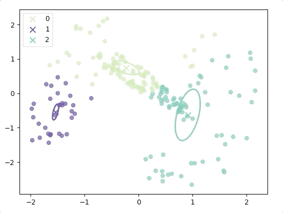
The progress of EM(initial with K-means):

and the final result is:

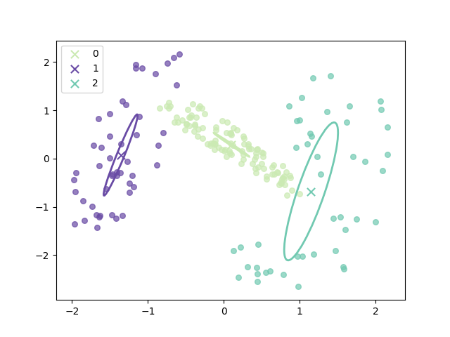
where the ellipse represents the covariance matrix and the axes of the ellipse are in the direction of eigenvectors of the covariance matrix, and their length is corresponding eigenvalues.

References

Bishop, Christopher M. Pattern recognition and machine learning. springer, 2006.↩︎