Discriminant Functions and Decision Boundary

Preliminaries

1. convex definition
2. linear algebra

• vector length
• vector direction

Discriminant Function in Classification

The discriminant function or discriminant model is on the other side of the generative model. And we, here, have a look at the behavior of the discriminant function in linear classification.¹

In the post ‘Least Squares Classification’, we have seen, in a linear classification task, the decision boundary is a line or hyperplane by which we separate two classes. And if our model is based on the decision boundary or, in other words, we separate inputs by a function and a threshold, the model is a discriminant model and the decision boundary is formed by the function and a threshold.

Now, we are going to talk about what the decision boundaries look like in the \(K\)-classes problem when \(K=2\) and \(K>2\). To illustrate the boundaries, we only consider the 2D(two dimensional) input vector \(\mathbf{x}\) who has only two components.

Two classes

The easiest decision boundary comes from 2-dimensional input space which is separated into 2 regions:

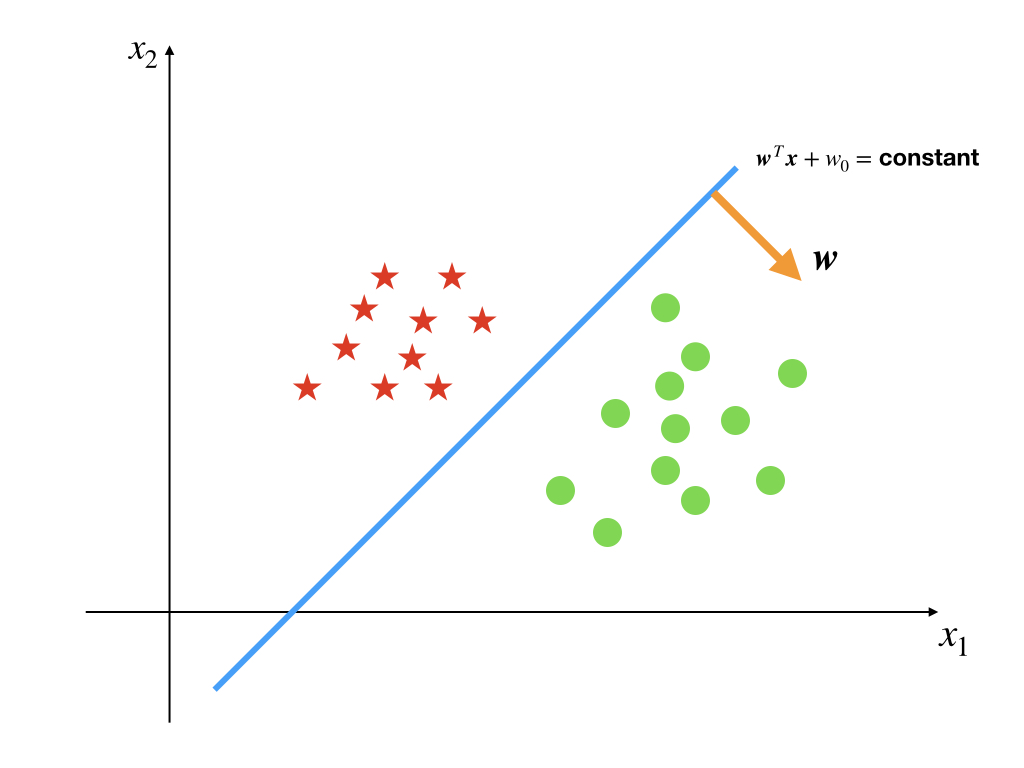
whose decision boundary is:

\[ \mathbf{w}^T\mathbf{x}+w_0=\text{ constant }\tag{1} \]

This equation is equal to \(\mathbf{w}^T\mathbf{x}+w_0=0\) because \(w_0\) is also a constant, so it can be merged with the r.h.s. constant. Of course, the 1-dimensional input space is easier than 2-dimensional, and its decision boundary is a point.

Let’s go back to the line, and it has the following properties:

1. The vector \(\mathbf{w}\) always points to a certain region and is perpendicular to the line.
2. \(w_0\) decides the location of the boundary relative to the origin.
3. The perpendicular distance \(r\) to the line of a point \(\mathbf{x}\) can be calculated by \(r=\frac{y(\mathbf{x})}{||\mathbf{w}||}\) where \(y(\mathbf{x})=\mathbf{w}^T\mathbf{x}+w_0\)

Because these three properties are all basic concepts of a line, we just prove the third point roughly:

proof: We set \(\mathbf{x}_{\perp}\) is the projection of \(\mathbf{x}\) on the line.

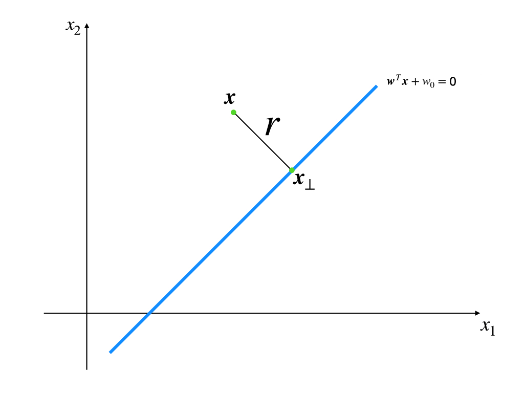
We using the first point that \(\mathbf{w}\) is perpendicular to the line and \(\frac{\mathbf{w}}{||\mathbf{w}||}\) is the union vector:

\[ \mathbf{x}=\mathbf{x}_{\perp}+r\frac{\mathbf{w}}{||\mathbf{w}||}\tag{2} \]

and we substitute equation (2) to the line function \(y(\mathbf{x})=\mathbf{w}^T\mathbf{x}+w_0\) :

\[ \begin{aligned} y(\mathbf{x})&=\mathbf{w}^T(\mathbf{x}_{\perp}+r\frac{\mathbf{w}}{||\mathbf{w}||})+w_0\\ &=\mathbf{w}^T\mathbf{x}_{\perp}+\mathbf{w}^Tr\frac{\mathbf{w}}{||\mathbf{w}||}+w_0\\ &=\mathbf{w}^Tr\frac{\mathbf{w}}{||\mathbf{w}||}\\ &=r\frac{||\mathbf{w}||^2}{||\mathbf{w}||}\\ \end{aligned}\tag{3} \]

So we have

\[ r=\frac{y(\mathbf{x})}{||\mathbf{w}||}\tag{4} \]

Q.E.D.

However, augmented vectors \(\mathbf{w}= \begin{bmatrix}w_0&w_1& \cdots&w_d\end{bmatrix}^T\) and \(\mathbf{x}= \begin{bmatrix}1&x_1& \cdots&x_d\end{bmatrix}^T\) can cancel \(w_0\) of the original boundary equation. So a \(d+1\)-dimensional hyperplane that went through the origin could be instea replaced by an \(d\)-dimensional hyperplane.

Multiple Classes

Things changed when we consider more than 2 classes. Their boundaries become more complicated, and we have 3 different strategies for this problem intuitively:

1-versus-the-rest Classifier

This strategy needs at least \(K-1\) classifiers(boundaries). Each classifier \(k\) just decides which side belongs to class \(k\) and the other side does not belong to \(k\). So when we have two boundaries, like:

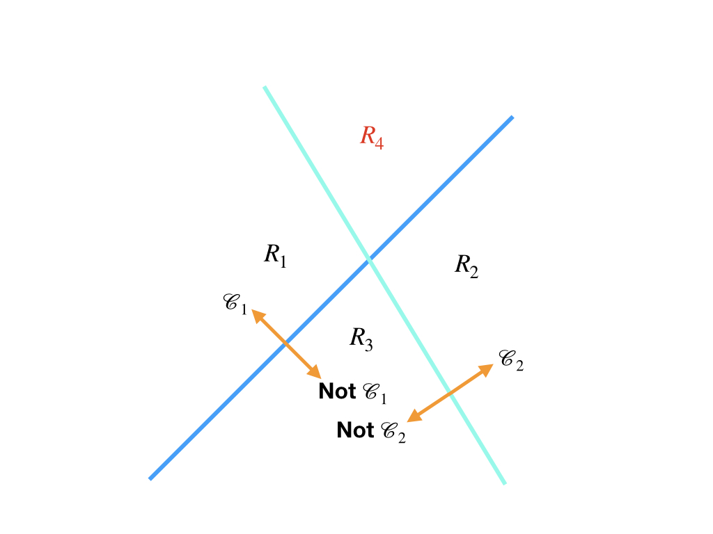
where the region \(R_4\) is embarrassed, based on the properties of the decision boundary, and the definition of classification in the post‘From Linear Regression to Linear Classification’, region \(R_4\) can not belong to \(\mathcal{C}_1\) and \(\mathbb{C}_2\) simultaneously.

So the first strategy can work for some regions, but there are some black whole regions where the input \(\mathbf{x}\) belongs to more than one class and some white whole regions where the input \(\mathbf{x}\) belongs to no classes(region \(R_3\) could be such a region)

1-versus-1 classifier

Another kind of multiple class boundary is the combination of several 1-versus-1 linear decision boundaries. Both sides of a decision boundary belong to a certain class, not like the 1-versus-rest classifier. And to a \(K\) class task, it needs \(K(K-1)/2\) binary discriminant functions.

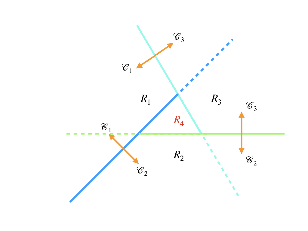
However, the contradiction still exists. Region \(R_4\) belongs to class \(\mathcal{C}_1\), \(\mathcal{C}_2\), and \(\mathcal{C}_3\) simultaneously.

So this is also not good for all situations.

\(K\) Linear functions

We use a set of \(K\) linear functions: \[ \begin{aligned} y_1(\mathbf{x})&=\mathbf{w}^T_1\mathbf{x}+w_{10}\\ y_2(\mathbf{x})&=\mathbf{w}^T_2\mathbf{x}+w_{20}\\ &\vdots \\ y_K(\mathbf{x})&=\mathbf{w}^T_K\mathbf{x}+w_{K0}\\ \end{aligned}\tag{5} \]

and an input belongs to \(k\) when \(y_k(\mathbf{x})>y_j(\mathbf{x})\) where \(j\in \{1,2,\cdots,K\}\) that \(j\neq k\). According to this definition, the decision boundary between class \(k\) and class \(j\) is \(y_k(\mathbf{x})=y_j(\mathbf{x})\) where \(k,j\in\{1,2,\cdots,K\}\) and \(j\neq k\). Then a decision hyperplane is defined as:

\[ (\mathbf{w}_k-\mathbf{w}_j)^T\mathbf{x}+(w_{k0}-w_{j0})=0\tag{6} \]

These decision boundaries separate the input spaces into \(K\) single connect, convex regions.

proof: choose two points in the region \(k\) that \(k\in \{1,2,\cdots,K\}\). \(\mathbf{x}_A\) and \(\mathbf{x}_B\) are two points in the region. An arbitrary point on the line between \(\mathbf{x}_A\) and \(\mathbf{x}_B\) can be written as \(\mathbf{x}'=\lambda \mathbf{x}_A + (1-\lambda)\mathbf{x}_B\) where \(0\leq\lambda\leq1\). For the linearity of \(y_k(\mathbf{x})\) we have:

\[ y_k(\mathbf{x}')=\lambda y_k(\mathbf{x}_A) + (1-\lambda)y_k(\mathbf{x}_B)\tag{7} \]

Because \(\mathbf{x}_A\) and \(\mathbf{x}_B\) belong to class \(k\), \(y_k(\mathbf{x}_A)>y_j(\mathbf{x}_A)\) and \(y_k(\mathbf{x}_B)>y_j(\mathbf{x}_B)\) where \(j\neq k\). Then \(y_k(\mathbf{x}')>y_j(\mathbf{x}')\) and the region of class \(k\) is convex.

Q.E.D

The last strategy seems good. And what we should do is estimate the parameters of the model. The most famous approaches that will study are: 1. Least square 2. Fisher’s linear discriminant 3. Perceptron algorithm

References

Bishop, Christopher M. Pattern recognition and machine learning. springer, 2006.↩︎