An Introduction to Probabilistic Generative Models

Preliminaries

1. Probability

• Bayesian Formular

2. Calculus

Probabilistic Generative Models¹

The generative model used for making decisions contains an inference step and a decision step:

1. Inference step is to calculate \(\Pr(\mathcal{C}_k|\mathbf{x})\) which means the probability of \(\mathbf{x}\) belonging to the class \(\mathcal{C}_k\) given \(\mathbf{x}\)
2. Decision step is to make a decision based on \(\Pr(\mathcal{C}_k|\mathbf{x})\) which was calculated in step 1

In this post, we just give an introduction and a framework for the probabilistic generative model in classification. But the details of how to estimate the parameters in the model will not be introduced.

From Bayesian Formular to Logistic Sigmoid Function

To build \(\Pr(\mathcal{C}_k|\mathbf{x})\), we can start from Bayesian formula. To the class \(\mathcal{C}_1\) of a two-classes problem, the posterior probability:

\[ \begin{aligned} \Pr(\mathcal{C}_1|\mathbf{x})&=\frac{\Pr(\mathbf{x}|\mathcal{C}_1)\Pr(\mathcal{C}_1)}{\Pr(\mathbf{x}|\mathcal{C}_1)\Pr(\mathcal{C}_1)+\Pr(\mathbf{x}|\mathcal{C}_2)\Pr(\mathcal{C}_2)}\\ &=\frac{1}{1+\frac{\Pr(\mathbf{x}|\mathcal{C}_2)\Pr(\mathcal{C}_2)}{\Pr(\mathbf{x}|\mathcal{C}_1)\Pr(\mathcal{C}_1)}} \end{aligned}\tag{1} \]

represents a new function:

\[ \begin{aligned} \Pr(\mathcal{C}_1|\mathbf{x})&=\delta(a)\\ &=\frac{1}{1+e^{-a}} \end{aligned}\tag{2} \]

where:

\[ a=\ln\frac{\Pr(\mathbf{x}|\mathcal{C}_1)\Pr(\mathcal{C}_1)}{\Pr(\mathbf{x}|\mathcal{C}_2)\Pr(\mathcal{C}_2)}\tag{3} \]

An usual question is why we set \(a=\ln\frac{\Pr(\mathbf{x}|\mathcal{C}_1)\Pr(\mathcal{C}_1)}{\Pr(\mathbf{x}|\mathcal{C}_2)\Pr(\mathcal{C}_2)}\) but not \(a=\ln\frac{\Pr(\mathbf{x}|\mathcal{C}_2)\Pr(\mathcal{C}_2)}{\Pr(\mathbf{x}|\mathcal{C}_1)\Pr(\mathcal{C}_1)}\). In my opinion, this \(a\) just determine the graph of function \(\delta(a)\). However, we perfer monotone-increasing function and \(\frac{1}{1+e^{-a}}\) is just a monotone-increasing function but \(\frac{1}{1+e^{a}}\) is not.

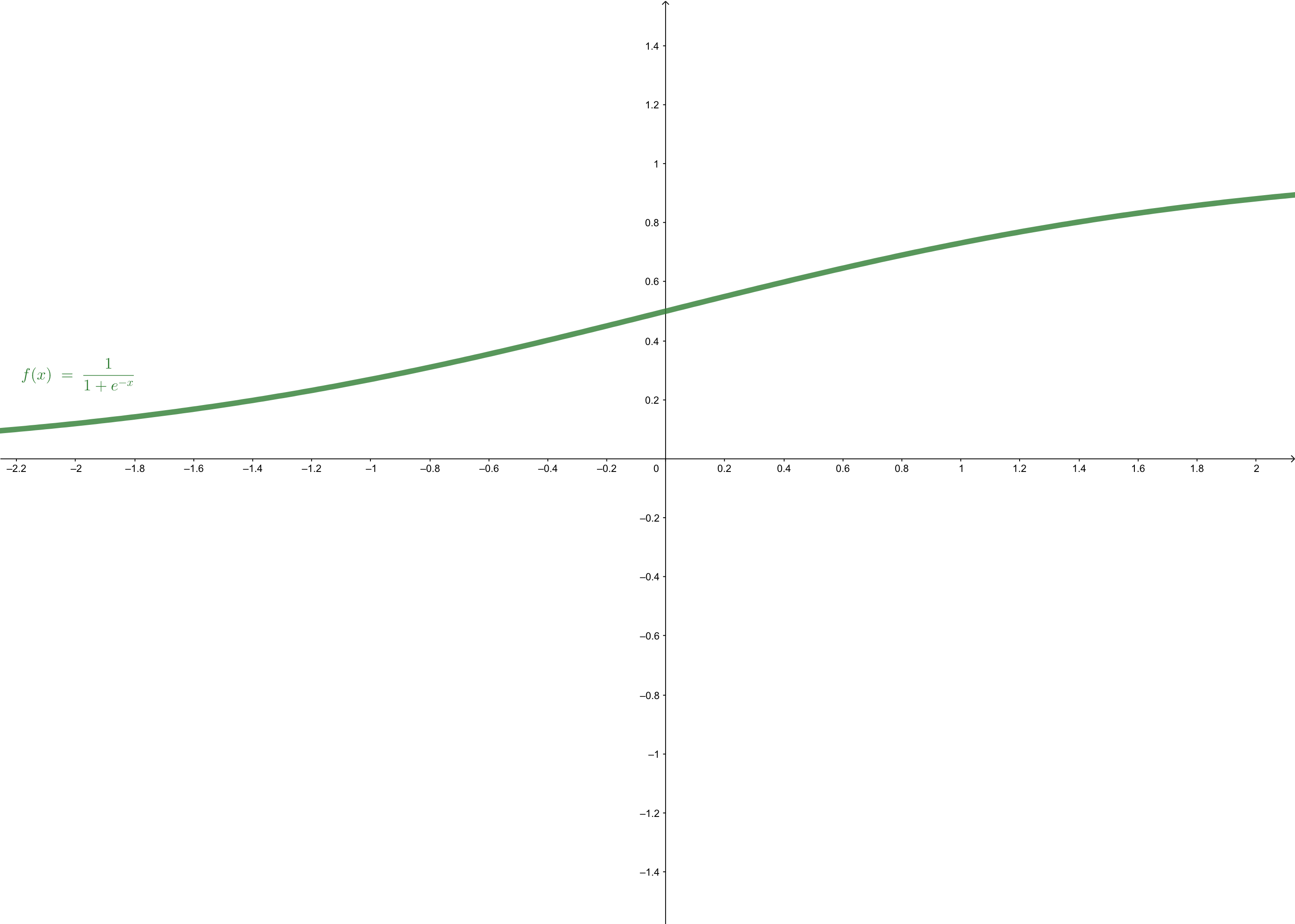
\(\delta(\cdot)\) is called logistic sigmoid function or squashing function, because it maps any number into interval \((0,1)\). The range of the function is just within the range of probability. So it is a good way to represent some kinds of probability, such as the \(\Pr(\mathcal{C}_1|\mathbf{x})\). the shape of the logistic sigmoid function is:

Some Properties of Logistic Sigmoid

For the logistic sigmoid function is symmetrical, then:

\[ 1-\delta(a)=\frac{e^{-a}}{1+e^{-a}}=\frac{1}{e^a+1}\tag{4} \]

and:

\[ \delta(-a)=\frac{1}{1+e^a}\tag{5} \]

So, we have an important equation:

\[ 1-\delta(a)=\delta(-a)\tag{6} \]

The inverse function of \(y=\delta(a)\) is: \[ \begin{aligned} y&=\frac{1}{1+e^{-a}}\\ e^{-a}&=\frac{1}{y}-1\\ a&=-\ln(\frac{1-y}{y})\\ a&=\ln(\frac{y}{1-y}) \end{aligned}\tag{7} \]

The derivative of the logistic sigmoid function is: \[ \frac{d\delta(a)}{d a}=\frac{e^{-a}}{(1+e^{-a})^2}=(1-\delta(a))\delta(a)\tag{8} \]

Multiple Classes Problems

We, now, extend the logistic sigmoid function into multiple classes condition. And we also start from the Bayesian formula:

\[ \Pr(\mathcal{C}_k|\mathbf{x})=\frac{\Pr(\mathbf{x}|\mathcal{C}_k)\Pr(\mathcal{C}_k)}{\sum_i\Pr(\mathbf{x}|\mathcal{C}_i)\Pr(\mathcal{C}_i)}\tag{9} \]

In this condition,if we set \(a_i=\ln\frac{\Pr(\mathbf{x}|\mathcal{C}_k)\Pr(\mathcal{C}_k)}{\Pr(\mathbf{x}|\mathcal{C}_i)\Pr(\mathcal{C}_i)}\), the whole fomular will be too complecated. To simplify the equation, we just set:

\[ a_i=\ln \Pr(\mathbf{x}|\mathcal{C}_k)\Pr(\mathcal{C}_k)\tag{10} \]

and we get a function of posterior probability: \[ \Pr(\mathcal{C}_k|\mathbf{x})=\frac{e^{a_k}}{\sum_i e^{a_i}}\tag{11} \] And according to the property of probability, we get the value of function: \[ y(a)=\frac{e^{a_k}}{\sum_i e^{a_i}}\tag{12} \] belongs to interval \([0,1]\). And it is called the softmax function. Although according to equation (10), the domain of the definition of softmax function is \((-\infty,0]\), \(a\) can be any real number. It’s called softmax because it is a smooth version of the max function.

When \(a_k\gg a_j\) for \(k\neq j\), we have:

\[ \begin{aligned} \Pr(\mathbf{x}|\mathcal{C}_k)&\simeq1\\ \Pr(\mathbf{x}|\mathcal{C}_j)&\simeq0 \end{aligned} \]

So both the logistic sigmoid function and softmax function can be used to form generative classifiers, which gives a value to the decision step.

References

Bishop, Christopher M. Pattern recognition and machine learning. springer, 2006.↩︎