An Introduction to Mixture Models

Preliminaries

1. linear regression
2. Maximum Likelihood Estimation
3. Gaussian Distribution
4. Conditional Distribution

From Supervised to Unsupervised Learning¹

We have discussed many machine learning algorithms, including linear regression, linear classification, neural network models, and e.t.c, till now. However, most of them are supervised learning, which means a teacher is leading the models to bias toward a certain task. In these problems our attention was on the probability distribution of parameters given inputs, outputs, and models:

\[ \Pr(\mathbf{\theta}|\mathbf{x},\mathbf{y},M)\tag{1} \]

where \(\mathbf{\theta}\) is a vector of the parameters in the model \(M\) and \(\mathbf{x}\), \(\mathbf{y}\) are inputs vector and output vector respectively. As what Bayesian equation told us, we can maximize equation (1) by maximizing the likelihood. And the probability

\[ \Pr(\mathbf{y}|\mathbf{x},\mathbf{\theta},M)\tag{2} \]

is the important component of the method. More details about the maximum likelihood method can be found Maximum Likelihood Estimation.

In today’s discussion, another probability will come to our’s minds. If we have no information about the target in the training set, it is to say we have no teacher in the training stage. We concerned about:

\[ \Pr(\mathbf{x})\tag{3} \]

Our task, now, could not be called classification or regression anymore. It is referred to as ‘cluster’ which is a progress of identifying which group the data point belongs to. What we have here is just a set of training points \(\mathbf{x}\) without targets and the probability \(\Pr(\mathbf{x})\).

Although this probability equation (3) is over one random variable, it can be arbitrarily complex. And sometimes, bringing in another random variable as assistance and combining them could get a new distribution that is relatively more tractable. That is to say, a joint distribution of observed variable \(\mathbf{x}\) and another created random variable \(\mathbf{z}\) could be more clear than the original distribution of \(\mathbf{x}\). And sometimes under this combination, the conditional distribution of \(\mathbf{x}\) given \(\mathbf{z}\) is very clear, too.

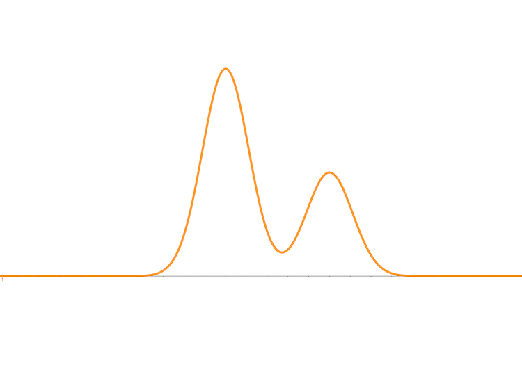
Let’s have look at a very simple example. \(\mathbf{x}\) has a distribution:

\[ a\cdot\exp(-\frac{(x-\mu_1)^2}{\delta_1})+b\cdot\exp(-\frac{(x-\mu_2)^2}{\delta_2})\tag{4} \]

where \(a\) and \(b\) are coeficients and \(\mu_1\), \(\mu_2\) are means of the Gaussian distributions and \(\delta_1\) and \(\delta_2\) are variances. It looks like this:

The random variable of equation (4) is just \(x\). However, now, we introduce another random variable \(z\in \{0,1\}\) as assistance into the distribution, in which \(z\) has a uniform distribution. Then the distribution (4) can be rewritten in a joint form:

\[ \Pr(x,z)=z\cdot a\cdot\exp(-\frac{(x-\mu_1)^2}{\delta_1})+(1-z)\cdot b\cdot\exp(-\frac{(x-\mu_2)^2}{\delta_2})\tag{5} \]

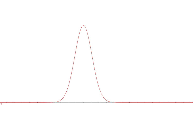
for \(\mathbf{z}\) is discrete random variable vector who has a uniform distribution so \(\Pr(z=0)=\Pr(z=1)=0.5\) and the conditional distribution is \(\Pr(x|z=1)\) is

\[ a\cdot\exp(-\frac{(x-\mu_1)^2}{\delta_1})\tag{6} \]

looks like:

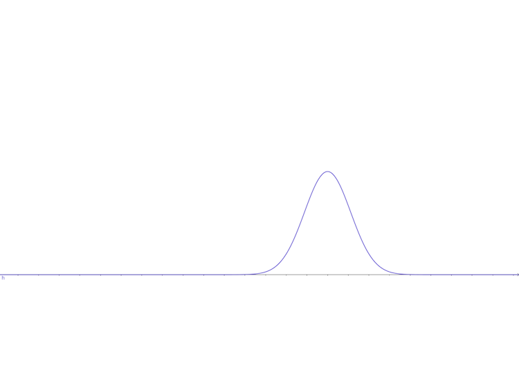
And the conditional distribution is \(\Pr(x|z=0)\) is \[ b\cdot\exp(-\frac{(x-\mu_2)^2}{\delta_2})\tag{7} \] looks like:

And the margin distribution of \(x\) is still equation (4)

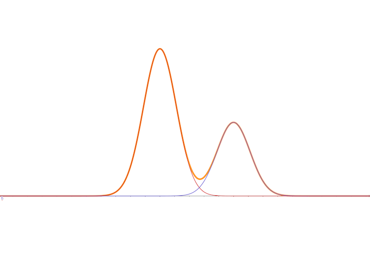
and its 3D vision is:

So the conditional distribution of \(x\) given \(z\) is just a single-variable Gaussian model, which is much simple to deal with. And so is the margin \(\Pr(x)\) by summing up all \(z\) (the rule of computing the margin distribution). Here the created random variable \(z\) is called a latent variable. It can be considered as an assistant input. However, it can also be considered as a kind of parameter of the model(we will discuss the details later). And the example above is the simplest Gaussian mixture which is wildly used in machine learning, statistics, and other fields. Here \(z\), the latent variable, is a discrete random variable, and the continuous latent variable will be introduced later as well.

Mixture distribution can be used to cluster data and what we are going to study are:

1. Non probabilistic version: K-means algorithm
2. Discrete latent variable and a relative algorithm which is known as EM algorithm

References

Bishop, Christopher M. Pattern recognition and machine learning. springer, 2006.↩︎