An Introduction to Linear Regression

Preliminariess

1. Linear Algebra(the concepts of space, vector)
2. Calculus

What is Linear Regression

Linear regression is a basic idea in statistical and machine learning based on the linear combination. And it was usually used to predict some responses to some inputs(predictors).

Machine Learning and Statistical Learning

Machine learning and statistical learning are similar but have some distinctions. In machine learning, models, regression models, or classification models, are used to predict the outputs of the new incoming inputs.

In contrast, in statistical learning, regression and classification are employed to model the data to find out the hidden relations among the inputs. In other words, the models of data, no matter they are regression or classification, or something else. They are used to analyze the mechanism behind the data.

“Linear”

Linear is a property of the operation \(f(\cdot)\), which has the following two properties:

1. \(f(a\mathbf{x})=af(\mathbf{x})\)
2. \(f(\mathbf{x}+\mathbf{y})=f(\mathbf{x})+f(\mathbf{y})\)

where \(a\) is a scalar. Then we say \(f(\cdot)\) is linear or \(f(\cdot)\) has a linearity property.

The linear operation can be represented as a matrix. And when a 2-dimensional linear operation was drawn on the paper, it is a line. Maybe that is why it is named linear, I guess.

“Regression”

In statistical or machine learning, regression is a crucial part of the whole field. And, the other part is the well-known classification. If we have a close look at the outputs data type, one distinction between them is that the output of regression is continuous but the output of classification is discrete.

What is linear regression

Linear regression is a regression model. All parameters in the model are linear, like:

\[ f(\mathbf{x})=w_1x_1+w_2x_2+w_3x_3\tag{1} \]

where the \(w_n\) where \(n=1,2,3\) are the parameters of the model, the output \(f(\mathbf{x})\) can be written as \(t\) for 1-deminsional outputs (or \(\mathbf{t}\) for multi-deminsional outputs).

\(f(\mathbf{w})\) is linear:

\[ \begin{aligned} f(a\cdot\mathbf{w})&=aw_1x_1+aw_2x_2+aw_3x_3=a\cdot f(\mathbf{w}) \\ f(\mathbf{w}+\mathbf{v})&=(w_1+v_1)x_1+(w_2+v_2)x_2+(w_3+v_3)x_3\\ &=w_1x_1+v_1x_1+w_2x_2+v_2x_2+w_3x_3+v_3x_3\\ &=f(\mathbf{w})+f(\mathbf{v}) \end{aligned}\tag{2} \]

where \(a\) is a scalar, and \(\mathbf{v}\) is in the same space with \(\mathbf{w}\)

Q.E.D

There is also another view that the linear property of models is also for \(\mathbf{x}\), the input.

But the following model

\[ t=f(\mathbf{x})=w_1\log(x_1)+w_2\sin(x_2)\tag{3} \]

is a case of linear regression problem in our definition. But from the second point of view, it is not linear for inputs \(\mathbf{x}\). However, this is not an unsolvable contradiction. If we use:

\[ y_1= \log(x_1)\\ y_2= \sin(x_2)\tag{4} \]

to replace the \(\log\) and \(\sin\) in equation (3), we get again

\[ t=f(\mathbf{y})=w_1y_1+w_2y_2\tag{5} \]

a linear operation for both input \(\mathbf{y}=\begin{bmatrix}y_1\;y_2\end{bmatrix}^T\) and parameters \(\mathbf{z}\) .

The tranformation, equation(4), is called feature extraction. \(\mathbf{y}\) is called features, and \(\log\) and \(\sin\) are called basis functions

An Example

This example is taken from (James2013¹), It is about the sale between different kinds of advertisements. I downloaded the data set from http://faculty.marshall.usc.edu/gareth-james/ISL/data.html. It’s a CSV file, including 200 rows. Here I draw 3 pictures using ‘matplotlib’ to make the data more visible. They are advertisements for ‘TV’, ‘Radio’, ‘Newspaper’ to ‘Sales’ respectively.

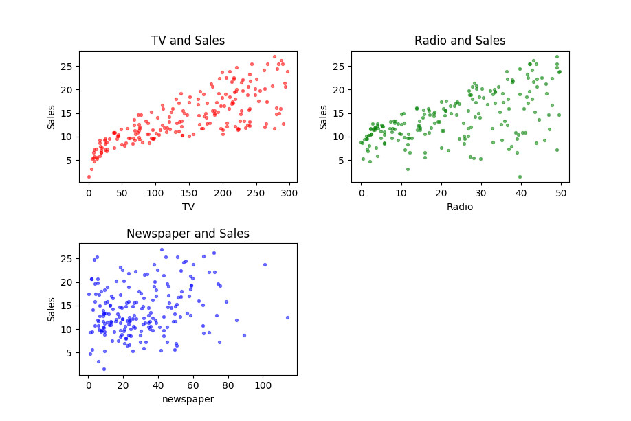
From these figures, we can find TV ads and Sales looks like having a stronger relationship than radio ads and sales. However, the Newspaper ads and Sales look independent.

For statistical learning, we should take statistical methods to investigate the relation in the data. And in machine learning, to a certain input, predicting an output is what we are concerned.

Why Linear Regression

Linear regression has been used for more than 200 years, and it’s always been our first class of statistical learning or machine learning. Here we list 3 practical elements of linear regression, which are essential for the whole subject:

1. It is still working in some areas. Although more complicated models have been built, they could not be replaced totally.
2. It is a good jump-off point to the other more feasible and adorable models, which may be an extension or generation of naive linear regression
3. Linear regression is easy, so it is possible to be analyzed mathematically.

This is why linear regression is always our first step to learn machine learning and statistical learning. And by now, this works pretty well.

A Probabilistic View

Machine learning or statistical learning can be described from two different views - Bayesian and Frequentist. They both worked well for some different instances, but they also have their limitations. The Bayesian view of the linear regression will be talked about as well later.

Bayesian statisticians thought the input \(\mathbf{x}\), the output \(t\), and the parameter \(\mathbf{w}\) are all random variables, while the frequentist does not think so. Bayesian statisticians predict the unknown input \(\mathbf{x}_0\) by forming the distribution \(\mathbb{P}(t_0|\mathbf{x}_0)\) and then sampling from it. To achieve this goal, we must build the \(\mathbb{P}(t|\mathbf{x})\) firstly. This is the modeling progress, or we can call it learning progress.

References

James, Gareth, Daniela Witten, Trevor Hastie, and Robert Tibshirani. An introduction to statistical learning. Vol. 112. New York: springer, 2013.↩︎