Preliminaries
Form LMS to Backpropagation1
The LMS algorithm is a kind of ‘performance learning’. And we have studied several learning rules(algorithms) till now, such as ‘Perceptron learning rule’ and ‘Supervised Hebbian learning’. And they were based on the idea of the physical mechanism of biological neuron networks.
Then performance learning was represented. Because of its outstanding performance, we go further and further away from natural intelligence into performance learning.
LMS can only solve the classification task which is linear separable. And then backpropagation(BP for short) which is a generalization of the LMS algorithm was introduced for more complex problems. And backpropagation is also an approximation of the steepest descent algorithm. The performance index of the problem which was supposed to be solved by backpropagation was MSE.
The distinction between BP and LMS is how derivative is calculated: 1. 1-layer network: \(\frac{\partial e}{\partial w}\) is relatively easy to compute. 2. multiple-layer network: \(\frac{\partial e}{\partial w_{i,j}}\) is complex. The chain rule would be employed to deal with the multiple-layer network with nonlinear transfer functions.
Brief History of BP
Rosenblatt and Widrow found the disadvantage of a single-layer network is that it can only solve the linear separable tasks. So they brought up the multilayer network. However, they had not developed an efficient learning rule to train a multilayer network.
In 1974, the first procedure of training a multilayer network was introduced by Paul Werbos in his thesis. However, this thesis was not noticed by researchers. In 1985 and 1986, David Parker, Yann LeCun, and Geoffry Hilton proposed the BP algorithm respectively. And in 1986, the book David R. and James M. ‘Parallel Distributed Processing’ made the algorithm known widely.
In the following several posts we would like to investigate: 1. The capacity of the multilayer network 2. BP algorithm
Multilayer Perceptrons
Let’s consider the 3-layer network:
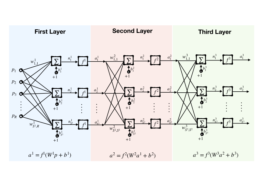
whose output is:
\[ \mathbf{a}^3=\mathbf{f}^3(W^3\mathbf{f}^2(W^2\mathbf{f}^1(W^1\mathbf{p}+\mathbf{b}^1)+\mathbf{b}^2)+\mathbf{b}^3) \]
and because all the outputs of one layer are inputs to the next layer and this makes it possible that the network can be notated as:
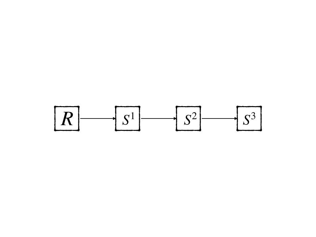
where \(R\) representes number of input and \(S^i\) for \(i=1,2,3\) is the number of neurons of layer 1,2,3.
We have now had the architecture of the new model multilayer network. What we should do next is to investigate the capacity of the multilayer network in:
- Pattern classification
- Function Approximation
Pattern Classification
Firstly, let’s have a look at a famous logical problem ‘exclusive-or’ or ‘XOR’ for short. This problem was famous for it can not be solved by a single-layer network which is proposed by Minsky and Papert in 1969.
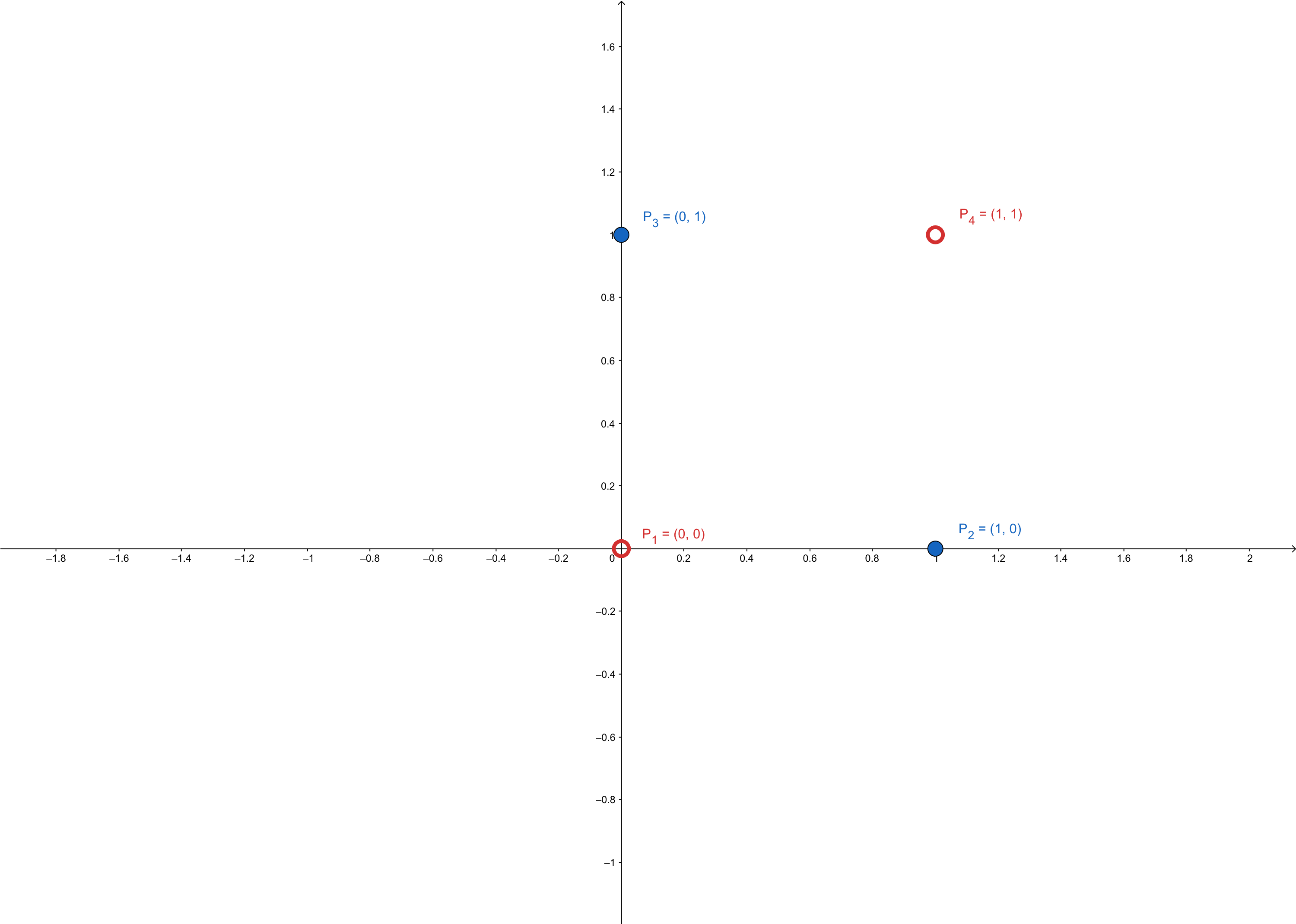
A Multilayer network was then invented to solve the ‘XOR’ problem. The input/output pairs of ‘XOR’ are
\[ \{\mathbf{p}_1=\begin{bmatrix} 0\\0 \end{bmatrix},\mathbf{t}_1=0\}\\ \{\mathbf{p}_2=\begin{bmatrix} 0\\1 \end{bmatrix},\mathbf{t}_2=1\}\\ \{\mathbf{p}_3=\begin{bmatrix} 1\\0 \end{bmatrix},\mathbf{t}_3=1\}\\ \{\mathbf{p}_4=\begin{bmatrix} 1\\1 \end{bmatrix},\mathbf{t}_4=0\} \]
and these points are not linear separable:
and if we use a 2-layer network, the XOR problem can be solved:
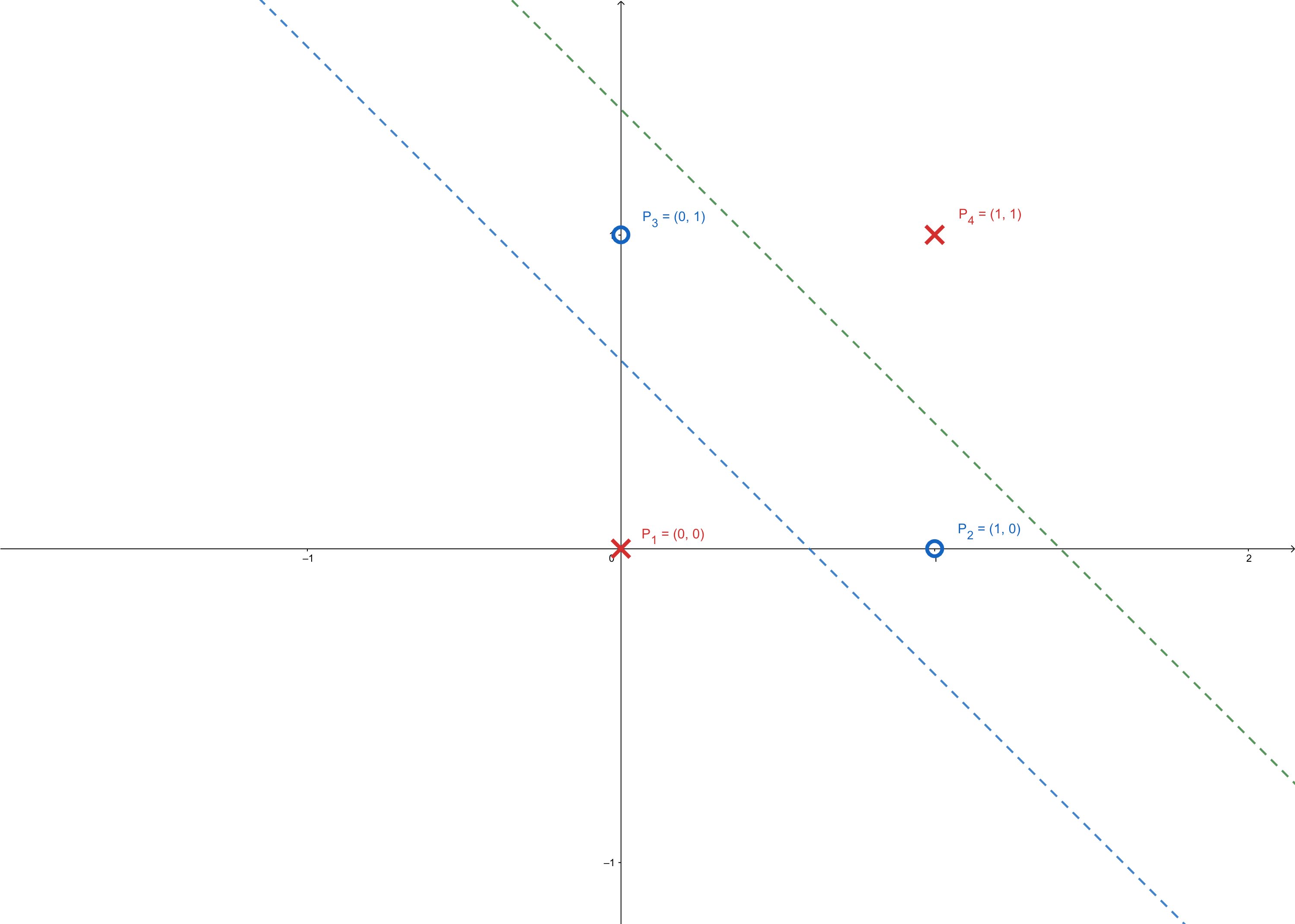
where these two lines can be constructed by two neurons:
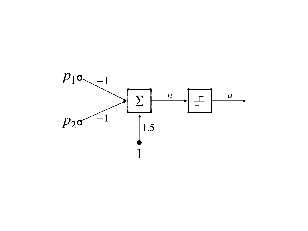
- The blue line can be \(y=-x+0.5\) and its neuron model is:

- The green line can be \(y=-x+1.5\) and its neuron model is:
And these two lines(neurons) can be mixed and constructed into a 2-layer network(2-2-1 network):
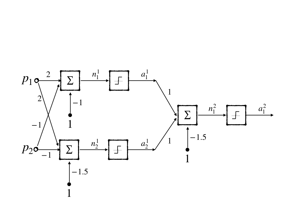
This gave a solution to the non-linear separable problem ‘XOR’. However, this is not a learning rule which means it could not be generalized to other more complex problems.
Function Approximation
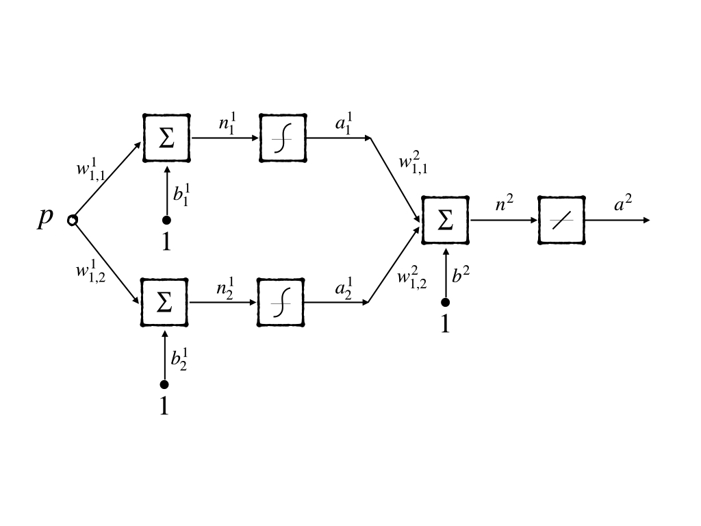
Besides classification, another task of the neuron network is function approximation. If we consider the intelligence of a model as an intricate function, the ability of the neuron network in approximating function should be studied. This capacity is also known as the model’s flexibility. Now let’s discuss the flexibility of a multilayer perceptron for implementing functions. A simple example is a good way to look inside of properties of a model without unnecessary details. So a ‘1-2-1’ network whose transfer function is logic-sigmoid in the first layer and linear function in the second layer is introduced:
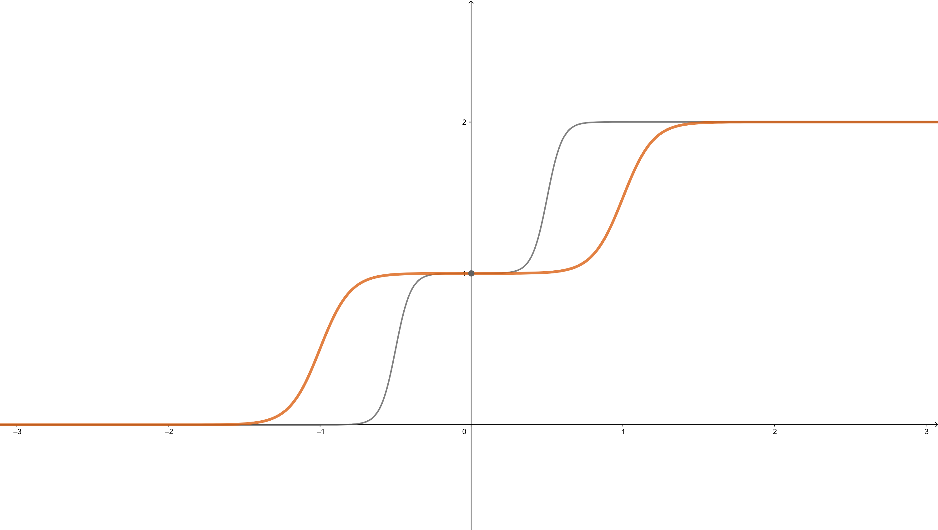
when \(w^1_{1,1}=10\), \(w^1_{2,1}=10\), \(b^1_1=-10\), \(b^1_2=10\), \(w^2_{1,1}=1\), \(w^2_{2,1}=1\), \(b^2=0\). It looks like:
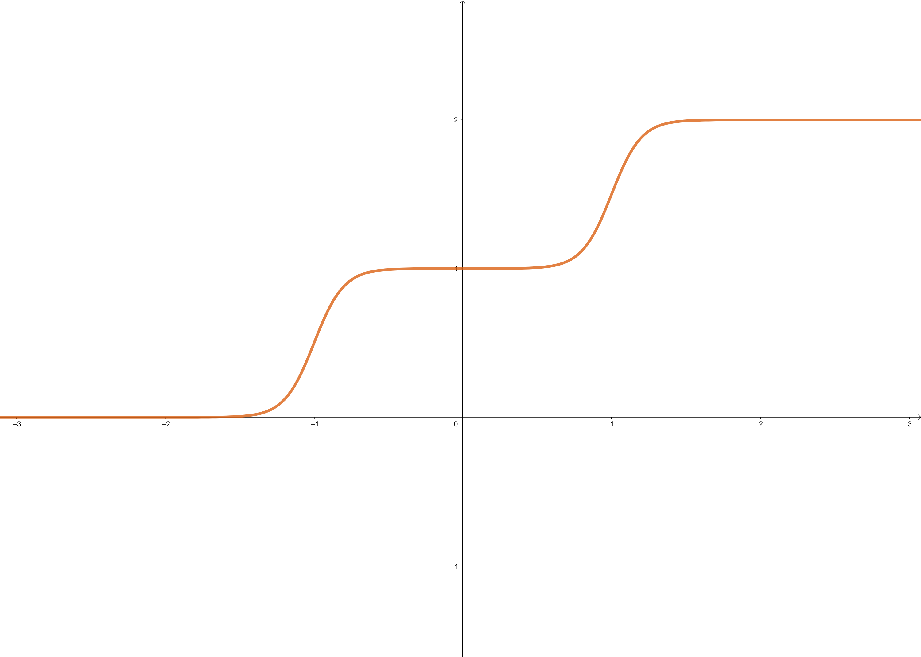
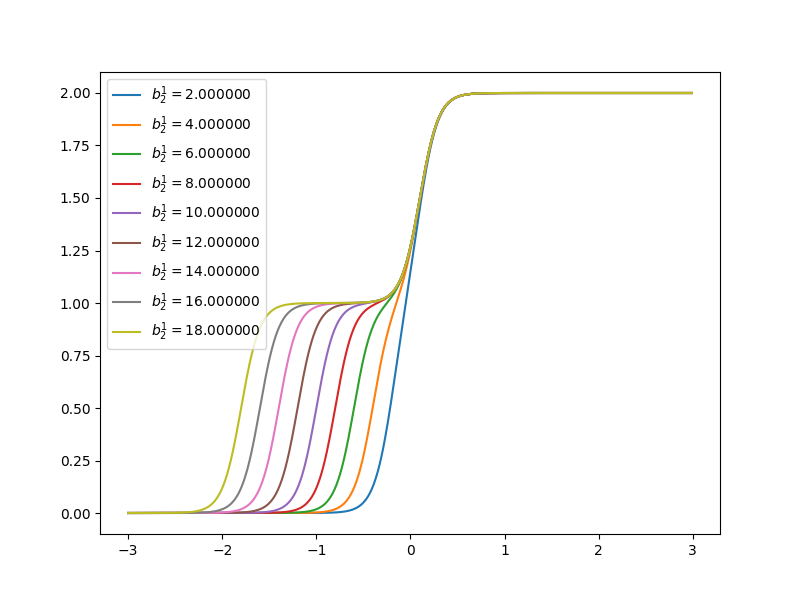
Each step can be changed by changing parameters. Because the steps are centered at
- \(n^1_1=0\) at \(p=1\)
- \(n^1_2=0\) at \(p=-1\)
and steps can be changed by changing weights. When \(w^1_{1,1}=20\), \(w^1_{2,1}=20\), \(b^1_1=-10\), \(b^1_2=10\), \(w^2_{1,1}=1\), \(w^2_{2,1}=1\), \(b^2=0\). It looks like the gray line in the figure:
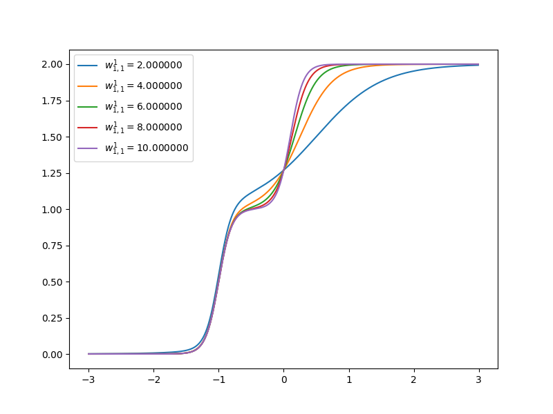
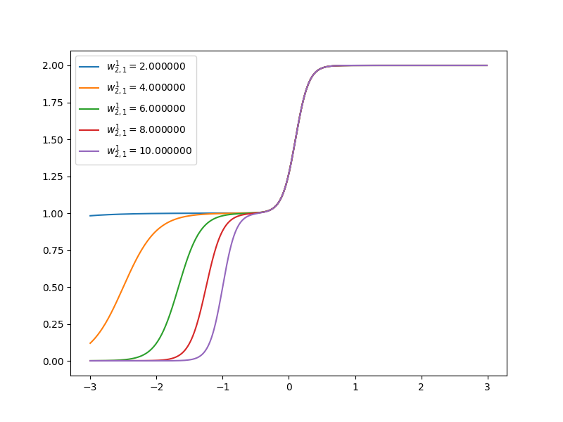
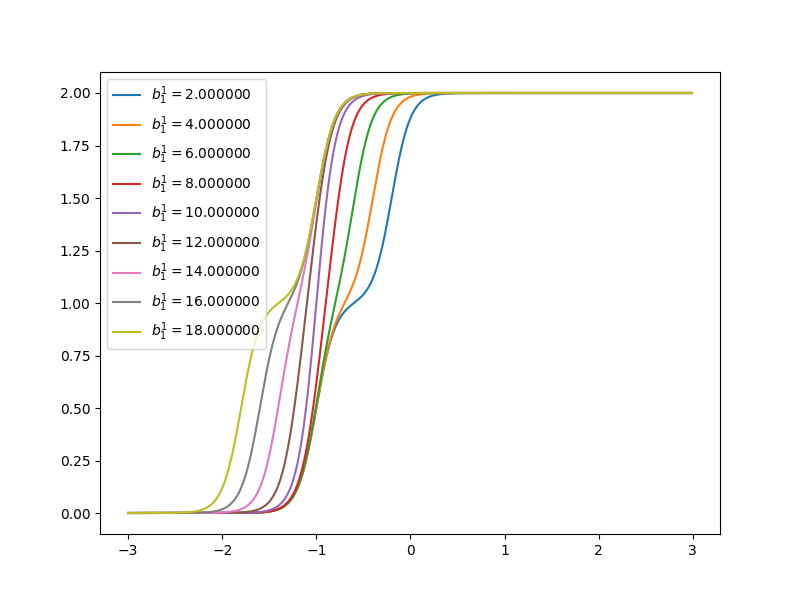
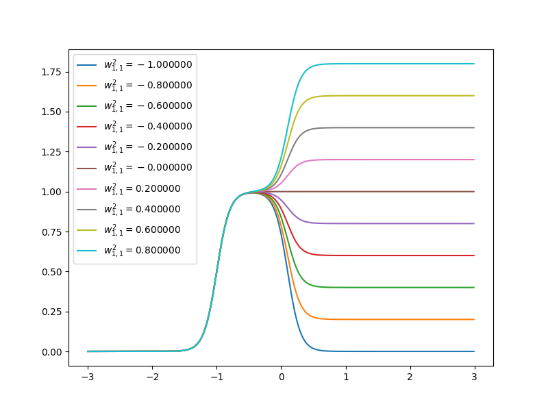
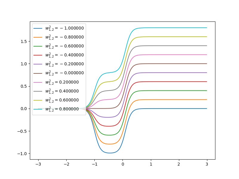
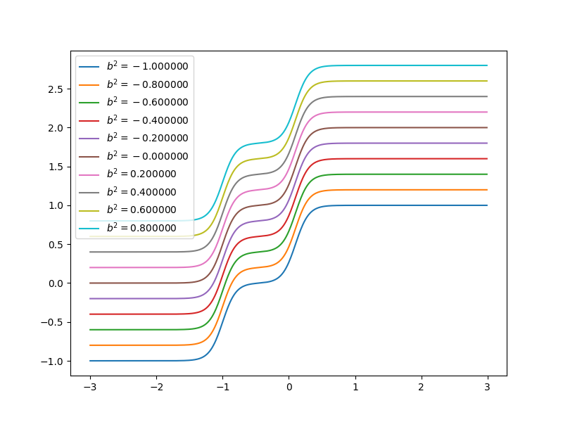
Now let’s have a look at how the curve of neuron networks looks like when one of the parameters is changing.
References
Demuth, Howard B., Mark H. Beale, Orlando De Jess, and Martin T. Hagan. Neural network design. Martin Hagan, 2014.↩︎