A Simple Linear Regression

Preliminaries

1. Linear Algebra(the concepts of space, vector)
2. Calculus
3. An Introduction to Linear Regression

Notations of Linear Regression¹

We have already created a simple linear model in the post “An Introduction to Linear Regression”. According to the definition of linearity, we can develop the simplest linear regression model:

\[ Y\sim w_1X+w_0\tag{1} \]

where the symbol \(\sim\) is read as “is approximately modeled as”. Equation (1) can also be described as “regressing \(Y\) on \(X\)(or \(Y\) onto \(X\))”.

Go back to the example that was given in “An Introduction to Linear Regression”. Combining with the equation (1), we get a model of the budget for TV advertisement and sales:

\[ \text{Sales}=w_1\times \text{TV}+ w_0\tag{2} \]

Assuming we have a machine here, which can turn grain into flour, the input is the grain, \(X\) in equation (1), and the output is flour, \(Y\). Accordingly, \(\mathbf{w}\) is the gears in the machine.

Then the mathematically model is:

\[ y=\hat{w_1}x+\hat{w_0}\tag{3} \]

The hat symbol “\(\;\hat{}\;\)” is used to present that this variable is a prediction, which means it is not the true value of the variable but a conjecture through certain mathematical strategies or methods else.

Then, a new input \(x_i\) has its prediction:

\[ \hat{y}_i=\hat{w_1}x_i+\hat{w_0}\tag{4} \]

Statistical learning mainly studies \(\begin{bmatrix}\hat{w_0}\\\hat{w_1}\end{bmatrix}\) but machine learning concerns more about \(\hat{y}\) All of them were based on the observed data.

Once we got this model, what we do next is estimating the parameters

Estimating the Parameters

For the advertisement task, what we have are a linear regression model equation(2) and a set of observations:

\[ \{(x_1,y_1),(x_2,y_2),(x_3,y_3),\dots,(x_n,y_n)\}\tag{5} \]

which is also known as training set. By the way, \(x_i\) in equation (5) is a sample of \(X\) and so is \(y_i\) of \(Y\). \(n\) is the size of the training set, the number of observations pairs.

The method we employed here is based on a measure of the “closeness” of the outputs of the model to the observed target (\(y\)s in set (5)). By far, the most used method is the “least squares criterion”.

The outputs \(\hat{y}_i\) of current model(parameters) to every input \(x_i\) are:

\[ \{(x_1,\hat{y}_1),(x_2,\hat{y}_2),(x_3,\hat{y}_3),\dots,(x_n,\hat{y}_n)\}\tag{6} \]

and the difference between \(\hat{y}_i\) and \(y_i\) is called residual and written as \(e_i\):

\[ e_i=y_i-\hat{y}_i\tag{7} \]

\(y_i\) is the target, which is the value our model is trying to achieve. So, the smaller the \(|e_i|\) is, the better the model is. Because the absolute operation is not a good analytic operation, we replace it with the quadratic operation:

\[ \mathcal{L}_\text{RSS}=e_1^2+e_2^2+\dots+e_n^2\tag{8} \]

\(\mathcal{L}_\text{RSS}\) means “Residual Sum of Squares”, the sum of total square residual. And to find a better model, we need to minimize the sum of the total residual. In machine learning, this is called loss function.

Now we take equations (4),(7) into (8):

\[ \begin{aligned} \mathcal{L}_\text{RSS}=&(y_1-\hat{w_1}x_1-\hat{w_0})^2+(y_2-\hat{w_1}x_2-\hat{w_0})^2+\\ &\dots+(y_n-\hat{w_1}x_n-\hat{w_0})^2\\ =&\sum_{i=1}^n(y_i-\hat{w_1}x_i-\hat{w_0})^2 \end{aligned}\tag{9} \]

To minimize the function “\(\mathcal{L}_\text{RSS}\)”, the calculus told us the possible minimum(maximum) points always stay at stationary points. And the stationary points are the points where the derivative of the function is zero. Remember that the minimum(maximum) points must be stationary points, but the stationary point is not necessary to be a minimum(maximum) point. For more information, ‘Numerical Optimization’ is a good book.

Since the ‘\(\mathcal{L}_\text{RSS}\)’ is a function of a vector \(\begin{bmatrix}w_0&w_1\end{bmatrix}^T\), the derivative is replaced by partial derivative. As the ‘\(\mathcal{L}_\text{RSS}\)’ is just a simple quadric surface, the minimum or maximum exists, and there is one and only one stationary point.

Then our mission to find the best parameters for the regression has been converted to calculus the solution of the function system that the derivative(partial derivative) is set to zero.

The partial derivative of \(\hat{w_1}\) is

\[ \begin{aligned} \frac{\partial{\mathcal{L}_\text{RSS}}}{\partial{\hat{w_1}}}=&-2\sum_{i=1}^nx_i(y_i-\hat{w_1}x_i-\hat{w_0})\\ =&-2(\sum_{i=1}^nx_iy_i-\hat{w_1}\sum_{i=1}^nx_i^2-\hat{w_0}\sum_{i=1}^nx_i) \end{aligned}\tag{10} \]

and derivative of \(\hat{w_0}\) is:

\[ \begin{aligned} \frac{\partial{\mathcal{L}_\text{RSS}}}{\partial{\hat{w_0}}}=&-2\sum_{i=1}^n(y_i-\hat{w_1}x_i-\hat{w_0})\\ =&-2(\sum_{i=1}^ny_i-\hat{w_1}\sum_{i=1}^nx_i-\sum_{i=1}^n\hat{w_0}) \end{aligned}\tag{11} \]

Set both of them to zero and we can get:

\[ \begin{aligned} \frac{\partial{\mathcal{L}_\text{RSS}}}{\partial{\hat{w_0}}}&=0\\ \hat{w_0} &=\frac{\sum_{i=1}^ny_i-\hat{w_1}\sum_{i=1}^nx_i}{n}\\ &=\bar{y}-\hat{w_1}\bar{x} \end{aligned}\tag{12} \]

and

\[ \begin{aligned} \frac{\partial{\mathcal{L}_\text{RSS}}}{\partial{\hat{w_1}}}&=0\\ \hat{w_1}&=\frac{\sum_{i=1}^nx_iy_i-\hat{w_0}\sum_{i=1}^nx_i}{\sum_{i=1}^nx_i^2} \end{aligned}\tag{13} \]

To get a equation of \(\hat{w_1}\) independently, we take equation(13) to equation(12):

\[ \begin{aligned} \frac{\partial{\mathcal{L}_\text{RSS}}}{\partial{\hat{w_1}}}&=0\\ \hat{w_1}&=\frac{\sum_{i=1}^nx_i(y_i-\bar{y})}{\sum_{i=1}^nx_i(x_i-\bar{x})} \end{aligned}\tag{14} \]

where \(\bar{x}=\frac{\sum_{i=1}^nx_i}{n}\) and \(\bar{y}=\frac{\sum_{i=1}^ny_i}{n}\)

By the way, equation (14) has another form:

\[ \hat{w_1}=\frac{\sum_{i=1}^n(x_i-\bar{x})(y_i-\bar{y})}{\sum_{i=1}^n(x_i-\bar{x})(x_i-\bar{x})}\tag{15} \]

and they are equal.

Diagrams and Code

Using python to demonstrate our result Equ. (12)(14) is correct:

import numpy as np
import pandas as pd
import matplotlib.pyplot as plt

# load data from csv file by pandas
AdvertisingFilepath='./data/Advertising.csv'
data=pd.read_csv(AdvertisingFilepath)

# convert original data to numpy array
data_TV=np.array(data['TV'])
data_sale=np.array(data['sales'])

# calculate mean of x and y
y_sum=0
y_mean=0
x_sum=0
x_mean=0
for x,y in zip(data_TV,data_sale):
    y_sum+=y
    x_sum+=x
if len(data_sale)!=0:
    y_mean=y_sum/len(data_sale)
if len(data_TV)!=0:
    x_mean=x_sum/len(data_TV)

# calculate w_1
w_1=0
a=0
b=0
for x,y in zip(data_TV,data_sale):
    a += x*(y-y_mean)
    b += x*(x-x_mean)
if b!=0:
    w_1=a/b

# calculate w_0
w_0=y_mean-w_1*x_mean

# draw a picture
plt.xlabel('TV')
plt.ylabel('Sales')
plt.title('TV and Sales')
plt.scatter(data_TV,data_sale,s=8,c='g', alpha=0.5)
x=np.arange(-10,350,0.1)
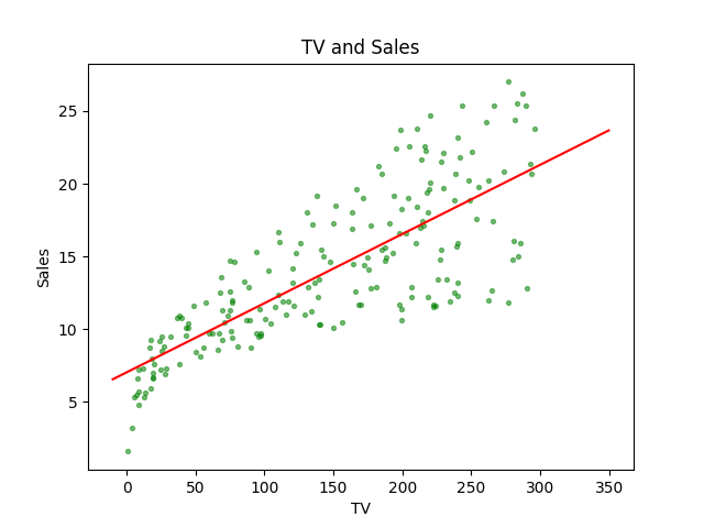
plt.plot(x,w_1*x+w_0,'r-')
plt.show()

After running the code, we got:

Reference